Header Image: Reddit: Snake Charmer _ Morocco_ 1950

Evolution

Pure Hand Colorization

Hand colorization is laborious and time consuming. The first film colorization methods were hand done by individuals. Now, some artists are still using manual colorization method to colorize old pictures. In Reddit, there are still some popular colorization forums, such as Colorization and ColorizedHistory.

For example, in order to colorize a still image an artist typically begins by segmenting the image into regions, and then proceeds to assign a color to each region. Thus, the artist is often left with the task of manually delineating complicated boundaries between regions. Colorization of movies requires, in addition, tracking regions across the frames of a shot. Existing tracking algorithms typically fail to robustly track non-rigid regions, again requiring massive user intervention in the process. ¹

It is worth mentioning that even though this is a labor intensive job and very expensive in making videos, the hand colorization can give the best colorization effect than any other (semi-)automatic techniques.

Scribble-Based Colorization

Unfortunately, automatic segmentation algorithms often fail to correctly identify fuzzy or complex region boundaries,such as the boundary between a subject’s hair and her face.

Colorization using Optimization

In 2004, Levin ¹ has proposed a new interactive colorization technique that requires neither precise manual segmentation, nor accurate tracking. The user indicates how each region should be colored by scribbling the desired color in the interior of the region, instead of tracing out its precise boundary.

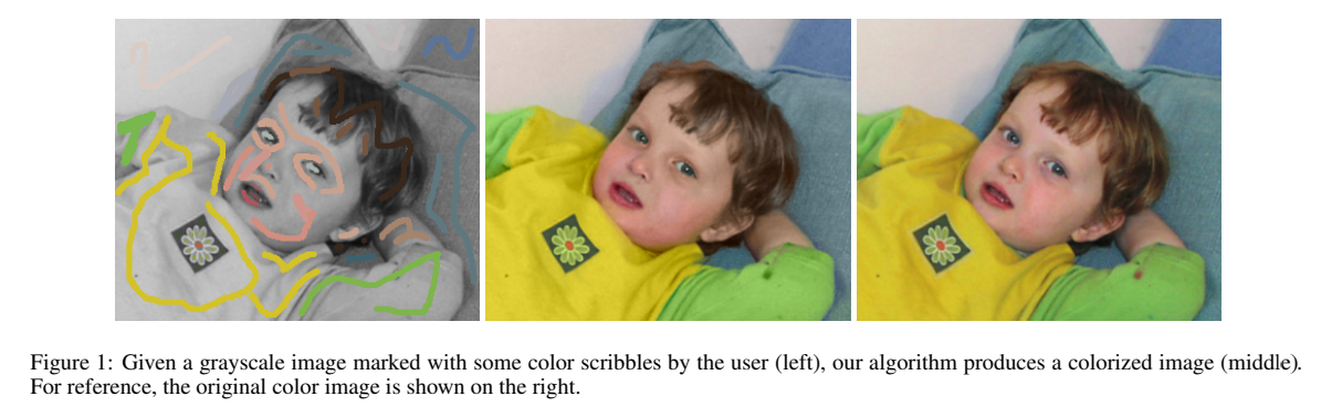
This algorithm is working in YUV color space, where \(Y\) is the monochromatic luminance channel, which we will refer to simply as intensity, while \(U\) and \(V\) are the chrominance channels, encoding the color. The algorithm is given as input an intensity volume \(Y(x,y,t)\) and outputs two color volumes \(U(x,y,t)\) and \(V(x,y,t)\).

Levin wished to impose the constraint that two neighboring pixels, r, s should have similar colors if their intensities are similar. Thus, to minimize the difference between the color U(r) at pixel r and the weighted average of the colors at neighboring pixels:

where \(w_{\boldsymbol{rs}}\) is a weighting function that sums to one, large when \(Y(\boldsymbol{r})\) is similar to \(Y(\boldsymbol{s})\), and small when the two intensities are different. Similar weighting functions are used extensively in image segmentation algorithms, where they are usually referred to as affinity functions.

He has experimented with two weighting functions. The simplest one is commonly used by image segmentation algorithms and is based on the squared difference between the two intensities:

A second weighting function is based on the normalized correlation between the two intensities:

where \(\mu_{\boldsymbol{r}}\) and \(\sigma_{\boldsymbol{r}}\) are the mean and variance of the intensities in a window around \(\boldsymbol{r}\).

The correlation affinity can also be derived from assuming a local linear relation between color and intensity. Formally, it assumes that the color at a pixel \(U(\boldsymbol{r})\) is a linear function of the intensity \(Y(\boldsymbol{r})\):

and the linear coefficients \(a_i, b_i\) are the same for all pixels in a small neighborhood around \(\boldsymbol{r}\). When the intensity is constant the color should be constant, and when the intensity is an edge the color should also be an edge.

The notation \(\boldsymbol{r} \in N(\boldsymbol{s})\) denotes the fact that \(\boldsymbol{r}\) and \(\boldsymbol{s}\) are neighboring pixels.

Now given a set of location \(\boldsymbol{r}_i\) where the colors are specified by the user \(u(\boldsymbol{r}_i)=u_i, v(\boldsymbol{r}_i)=v_i\) we minimize \(J(U), J(U)\) subject to these constraints. Since the cost functions are quadratic and the constraints are linear, this optimization problem yields a large, sparse system of linear equations, which may be solved using a number of standard methods.

The whole algorithm was done by solving a quadratic cost function derived from differences of intensities between a pixel and its neighboring pixels.

An Adaptive Edge Detection Based Colorization Algorithm and Its Applications

Huang ² has improved the method above to prevent the color bleeding over object boundaries.

Weighting Function

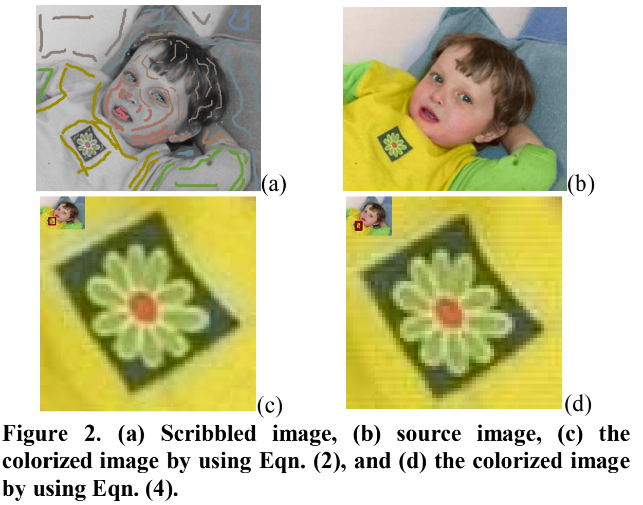
Huang has found that the two weighting functions do not always change the chrominance values proportional to the luminance similarities, so he proposed a new weighting function in the following:

where \(\boldsymbol{r}\) is a particular pixel, \(\boldsymbol{s}\) is one of the neighboring pixels of \(\boldsymbol{r}\), and \(Var(\boldsymbol{r})\) is the variance value of \(3 \times 3\) windowed pixels centered on \(\boldsymbol{r}\).

Adaptive Edge Detection Algorithm

They found that some colorized regions are blurred because different object colors propagating and interlacing together. The wrong colorization usually occurs near the cross borders of two objects.

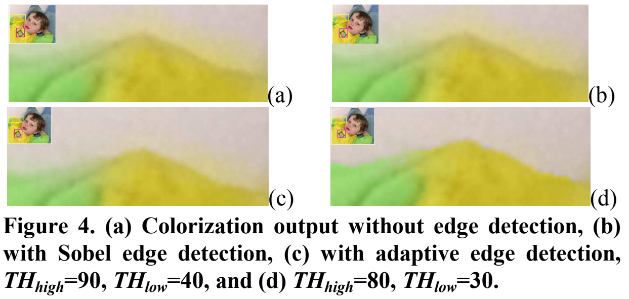
An adaptive edge detection scheme is proposed. First, they applied the Sobel filter with a high threshold, \(TH_{high}\), to the input grayscale image, which generate our initial edge map. Four kinds of Sobel filters adopted to detect horizontal, vertical, diagonal down-left, and opposite diagonal down-right edges, and the edge value, \(E_{Sum}\), is derived as follows:

Secondly, the pixels marked as edges will be extended with a lower threshold along the direction of the edge. The running threshold is decreased adaptively by a factor of 0.8 until a low bound, \(TH_{low}\) is reached. After all edge pixels in the initial map have gone through this extension process, we get an extended edge map.

Thirdly, for each pixel in the extended edge map we find the local maximum among its 8 neighboring pixels by comparing their Sobel filtering outputs. Each pixel is either marked as local maximum or having its own maximum direction. After that, linking these local maximums to extract edge skeletons. In this process, we sort all local maximums and try to link them to two of their neighboring maximums. There are still some broken edges because of their Sobel filtering results are not large enough or lower than \(TH_{low}\). We search in the extended edge map for a path to link these two extremities if they are not belonging to the same connected edge or of far distance along the edge.

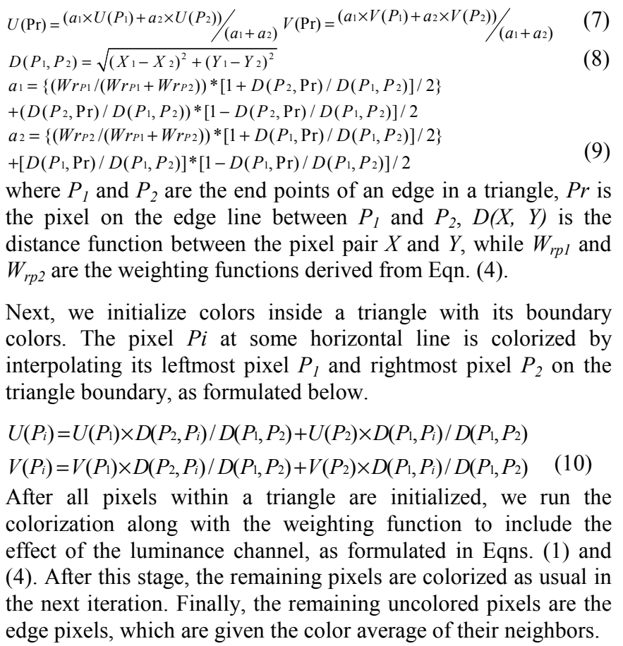
Non-Iterative

As shown in the figure above, color discontinuity will occur if only one iteration is allowed. The artifact originates from the independent color flooding from two different colors. If we can connect those discontinuously colorized pixels first and assign suitable colors to pixels on the connecting path, the discontinuity effect will be minimized. Thus, they triangulated the pixels that have been assigned with some specific colors in the same object region by the Delauney triangulation algorithm. Then, we colorize the edge lines of the triangle by using the following equations.

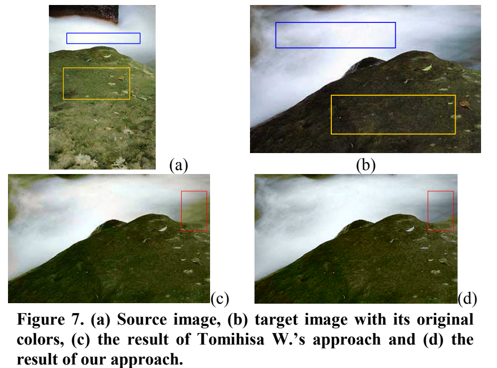
Fast Image and Video Colorization Using Chrominance Blending ³

Similarly to other colorization method, they use luminance/chrominance color systems, YCbCr. Moreover, work can be done also directly on the RGB space.

Let \(Y(x,y,\tau):\Omega \times [0, T) \rightarrow \mathcal{R}^+\) be the given monochromatic image \(T=0\) defined on a region \(\Omega\). Our goal is to complete the \(Cb\) and \(Cr\) channels respectively (same formula above). The proposed technique also uses as input observed values of the chrominance channels in a region \(\Omega_c \in \Omega \) which is significantly smaller than \(\Omega \). These values are often provided by the user or borrowed from other data.

Let \(s\) and \(t\) be two points in \(\Omega \) and let \(C(s):[0, 1] \rightarrow \frac{\Omega}{\Omega_c}\) be a curve in \(\Omega\). Let also \(C_{s,t}\) be a curve connecting \(s and t\) such that \(C(0)=s\) and \(C(1)=t\). We define the intrinsic (geodesic) distance between \(s and t\) by:

This intrinsic distance gives ameasurement of how “flat” is the flattest curve between any two points in the luminance channel.

A close relationship between the basic geometry of these channels is frequently observed in natural images. Sharp luminance changes are likely to indicate an edge in the chrominance, and a gradual change in luminance often indicates that the chrominance is also not likely to have an edge but rather a moderate change. From this, for the proposed colorization approach they assumed that the smaller the intrinsic distance \(d(s,t)\) between two points \((s,t)\) the more similar chrominance they would have.

We define the intrinsic distance from a certain chrominance \(c\) as the minimum distance from any point of the same chrominance \(c\) in \(\Omega_c\):

Their idea for colorization is to compute the Cb and Cr components of a point \(t\) in the region where they are missing \(\frac{\Omega}{\Omega_c}\) by blending the different chrominance in \(\Omega_c\) according to their intrinsic distance to \(t\):

where \(chrominances(A)\) stands for all the different unique chrominance in the region A and \(W(\cdot)\) is a function of the intrinsic distance that translates it into a blending weight. Some basic properties for \(W\):

\(1) \lim_{r\rightarrow 0}W(r)=\infty\\ 2) \lim_{r\rightarrow \infty}W(r)=0\\ 3) \lim_{d\rightarrow \infty}W(d+c)/W(d)=1\) Requirement 3 is necessary when there are two or more chrominance sources close-by but the blending is done relatively far from all sources. The desired visual result would even be the blending of all chrominance. For the experiments reported below we used

where \(b\) is the blending factor, typically \(1 \leq b \leq 6\). The factor defines how smooth is the chromnance transition.

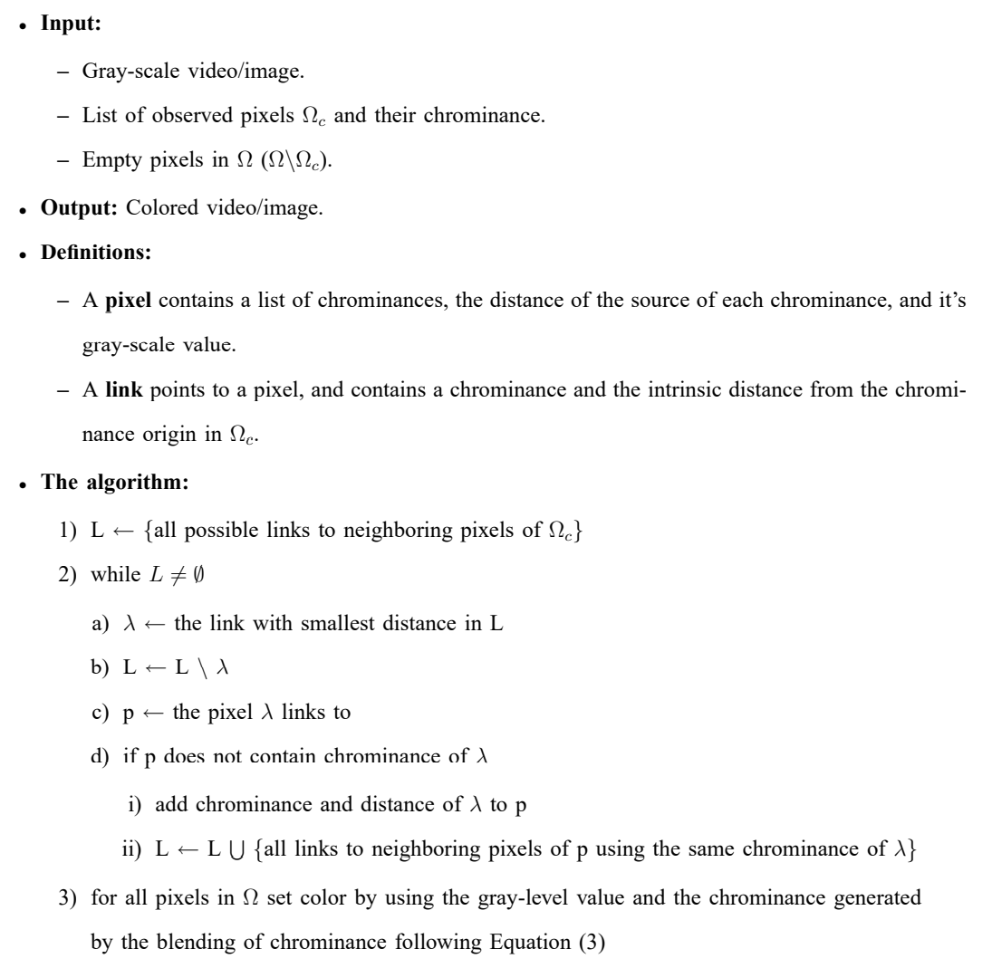
The whole algorithm is shown below.

Reference

• Wikipedia-Film-colorization

• Previous
  Colorization Insight Introduction
• Next
  Colorization Insight Scribbled 2