Header Image: Reddit: Young Ava Gardner
Evolution
Scribble-Based Colorization
Manga Colorization
Texture classification has also been used for cartoon colorization by Qu1.
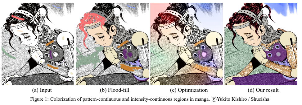
The whole process begins by a user scribbling on regions of interest. The system processes the user input incrementally. In each incremental step, the user enters one or more scribbles to segment the desired regions.
Two modes are provided by the system for segmentation, pattern-continuous and intensity-continuous propagations. It is up to the user to decide which mode of propagation should be employed in the current step. The pattern-continuous are designed for hatched/screened region and intensity-continuous propagation for intensity-continuous region with/without unclosed outlines.
Once the regions are segmented, they can be colorized using the proposed stroke-preserving colorization, pattern-to-shading, and multi-color transition, based on the user decision.
Hatching and Screening
Hatching and screening techniques are adopted to express various effects including shading, material reflectances, backgrounds, or even structures. While hatching mainly referes to hand-drawn strokes, screening makes use of printed comic pattern papers.
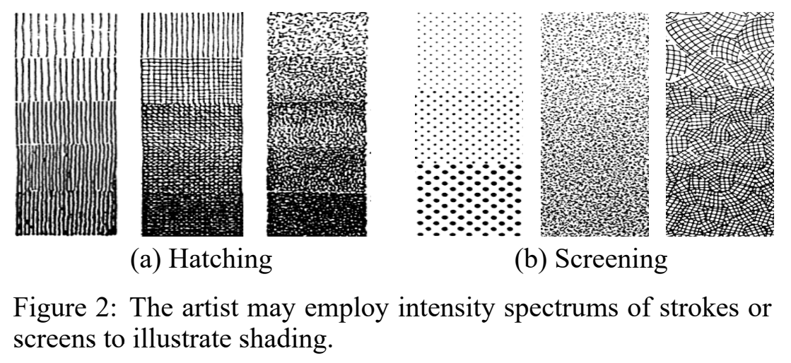
The change in gray level is abrupt in both hatching and screening.
Level Set
The level set method was employed due to its elegance in modeling multiple boundaries simultaneously. The geometric level set method is a zero surface method. The fundamental idea is to raise the modeling of boundaries from a two-dimensional planar curve into a three-dimensional curved surface, by embedding the propagating curves as the zero level set of a higher dimensional surface. This offers several advantages, including parameter-free representation, topological flexibility, and capability in dealing with local deformation. The colorization over both pattern-continuous and intensity-continuous regions can be naturally formulated under the same mathematical framework.
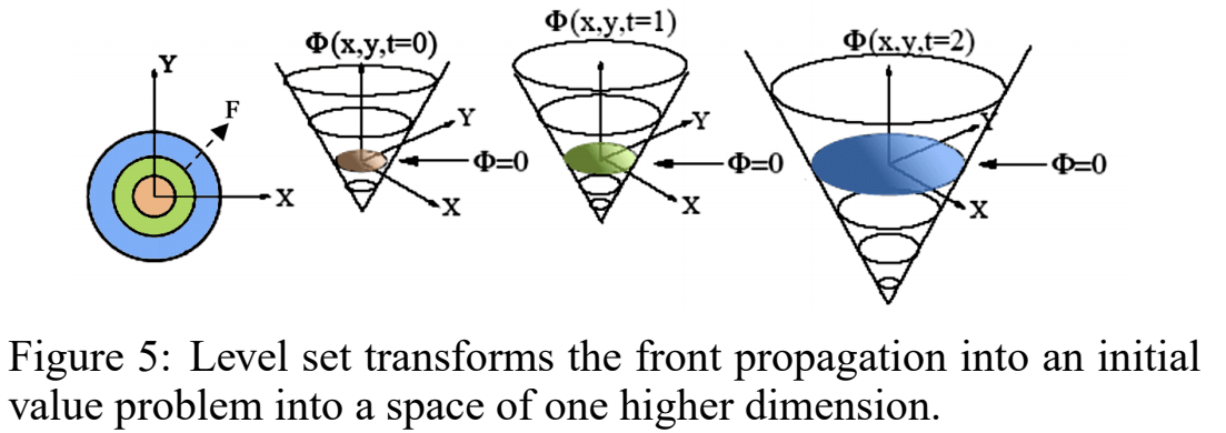
The level set method embeds the propagating curve \(T\) as the zero level set of an implicit function \(\Phi\) (i.e. the curve of \(\Phi=0\) ), which is defined over the entire image domain. As illustrated in figure below, the dimensionality of the level set function \(\Phi\) is one dimension higher than the evolving curve. In our case, \(\Phi\) is a 3D surface. The level set method tracks the evolution of a front that is moving normal to the boundary with a speed \(F(x,y)\). The speed function may be dependent on the local or global properties of the evolving boundary or driven by the external forces. Function \(\Phi\) is initialized based on a signed distance measured from the user scribble. The evolution of the boundary is defined by the partial differential equation on the zero level set of \(\Phi\):
\[\frac{\partial \Phi}{\partial t} = -F|\triangledown \Phi|\]where \(t\) is the time of evolution. The speed function \(F\) governs the actual behavior of the evolving boundary, including its movement and the stopping criteria.
For segmentation problems, the influence of the spped function F can be split into two major parts, \(F_A\) and \(F_G\). \(F_A\) is the positive advection term causing the front to uniformly expand. \(F_G\) depends on the geometry of the propagating front, such as local curvature. It controls the smoothness of the propagating front. Mathmatically,
\[\frac{\partial \Phi}{\partial t} = h \cdot (F_A+F_G)|\triangledown \Phi|\]where \(F_A\) is normally a constant; \(F_G=-\epsilon \kappa\) such that \(\kappa\) is the local curvature of the evolving curve \(T\) and \(\epsilon\) is a constant; \(h\) is a filter or halting component, to terminate the curve evolution.
The level set propagation starts by initializing \(\Phi\). In our application, we initialize \(\Phi\) as the signed distance from the user scribble. With \(\Phi\), the evolving curve \(T\) is naturally obtained (\(\Phi=0\)). A narrow band is constructed as the region surrounding \(T\) with a specified width. For each pixel within the narrow band, \(\Phi\) is updated according to Equation above. With this updated \(\Phi\), a new \(T\) can be computed. The iteration continues until convergence.
For more details about Pattern-continuous Region and Intensity-Continuous Regions, please refer to the paper1.
Colorization and Results
This paper demonstrates three ways to colorize these segmented areas.
Color Replacement
For the intensity-continuous region, filling color can be trivially done by replacing the black or white color by the user color on the scribble.
Stroke-Preserving Colorization
As mentioned before, the artist may use hatching/screening to express material reflectances, textures, or even shapes, it is sometimes necessary to preserve the original pattern during colorization. Instead of naively replacing the whole region with a single color, it is colorized by bleeding colors out of the strokes/patterns. The user color is multiplied with the halting term hI in the YUV space.
\[h_I(x,y) = \frac{1}{1+|\triangledown(G_{\sigma}\otimes I(x,y))|}\\ Y_{new}(x,y) = Y_{user} \otimes |1-h_I(x,y)|^2 \\ (U,V)_{new} = (U,V)_{user}\]where \(G_{\sigma}\otimes I(x,y)\) denotes convolution of the image \(I\) with a Gaussian smoothing filter \(G_{\sigma}\) with a characteristic width of \(\sigma\). \(h_I\) is a halting term that measures the change of intensity gradient. \(\otimes \) is the convolution operator.
Pattern to Shading
As color can readily reproduce such shading effect, we can convert the pattern to smooth color shading. In order to achieve this, we first calculate the local intensity within the pixel neighborhood,
\[s=f\otimes Y_{image}\]where \(f\) is a box filter. Note that \(s \in [0, 1]\). Then the Y channel is linearly mapped by
\[Y_{new} = sY_{user},\\ (U,V)_{new} = (U,V)_{user}\]Limitation
The proposed method has a limitation when two patterns overlap each other.
Natural Image Colorization
Luan2 employed texture similarity for more effective color propagation.
Traditional interactive scribble-based techniques require a very large number of strokes to achieve high quality colorization of images with complex textures.
Luan has proposed an interactive colorization system that requires modest amounts of user interactions for natural image colorization. Colrozation is explicitly divided into two steps in the system, Color Labeling and Color Mapping.
In the color labeling step, we designed a new labeling scheme to handle texture regions commonly seen in the natural images, in which not only nearby pixels with similar intensities but also remote pixels with similar texture features should share similar colors.This new framework makes it possible to segment natural images into coherent regions with a small number of strokes specified by the user.
In the color mapping step, colorization with rich color variation can be obtained using only a few color pixels assgined in the labeled region. We provide the user with realtime feedback so that he can simply select appropriate colors or create colorization of a variety of different styles.
Color Labeling
The objective of color labeling is to assign a color label to every pixel in the image, given the pseudo colors associated with user-drawn strokes.
Energy Optimization Framework
The textures should be explicitly taken into the consideration. One straightforward method is using the texture feature as the likelihood term in graphcut. However, erroneous labels may be brought in.
- The texture features at the highly contrastive locations tend to be well clustered in the feature space.
- The smooth regions are characterized by the coherence between neighboring colors, thus a pixel therein can be reliably colorized based on the intensity continuity.
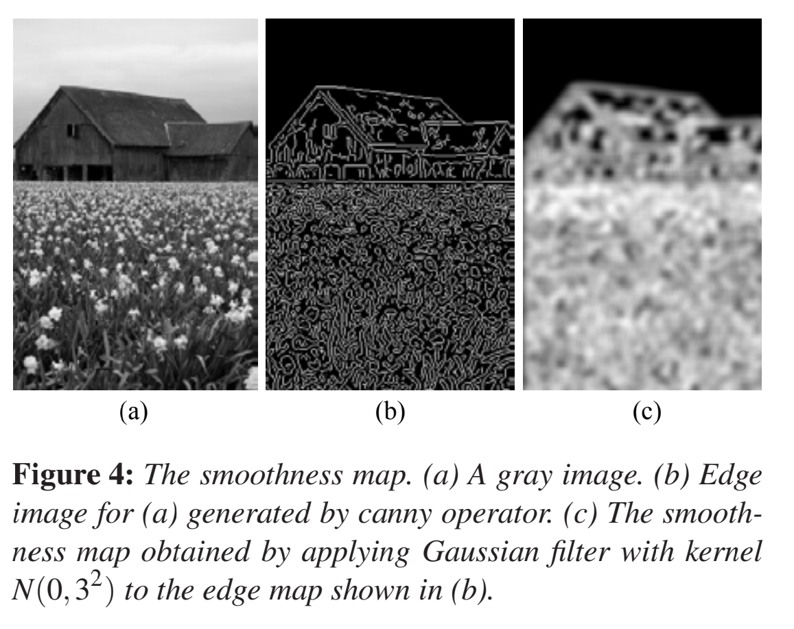
Motivated by the observation above, we propose a new formulation that integrates the intensity continuity and the texture-similarity. A smoothness value identifying different natures of locations is used to guide the incorporation of the two constraints. We trust more in the texture similarity term for highly contrastive locations, while the intensity continuity is considered as more reliable for smooth locations.
We obtain the likelihood of every pixel to be colored by each label color. This color label likelihood function is denoted as \(L(\mathbb{C};p)\), where \(\mathbb{C}\) represents all the label colors.
We introduce an energy optimization framework that incorporates both intensity continuity and texture similarity constraints for all the pixels \(p\) in the image:
\[E = \sum_{p\in img} (\lambda (p)E_1+(1-\lambda(p))E_2)\]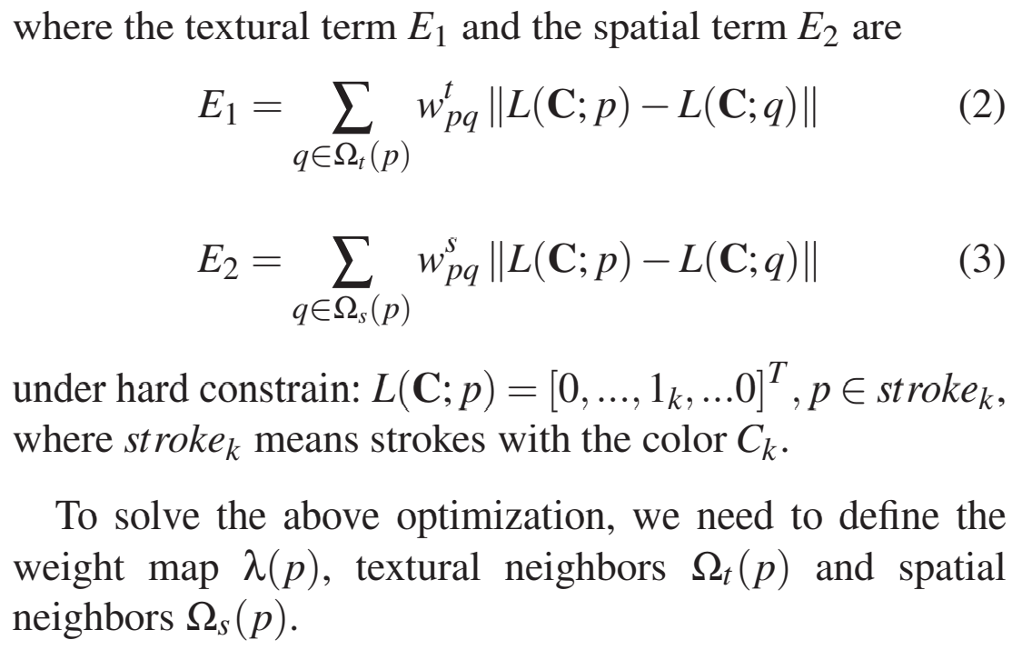
Smoothness Map: \(\lambda(p\))
In our method, we use the filtered edge map. At each pixel \(p\), the value of \(\lambda(p\)) is related to the distance between \(p\) to its nearest edge. Specifically, we use the Canny operator to extract the edges of the image. We then apply a Gaussian filter with kernel \(N(0,\sigma^2)\) on the edge image to obtain a smoothed edge map. If \(p\) is small. In our implementation, the \(\sigma\) is set as a quarter of the patch size that we used for texture space analysis.
Color Mapping
Once a region is selected, the user chooses a few pixels. These pixels represent a significant luminance variation in the region. Each pixel is then given a corresponding color by the user. The chroma (UV) values for any other pixels are then interpolated by piece-wise linear mapping in luminance (Y) space to get a color palette.
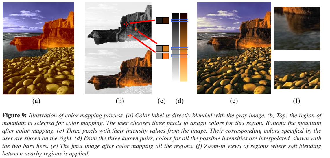
The final colorization result is not a hard composite of each colorized region. After colorizing the regions, we do a soft blending around the region boundary to make the color transition natural. Over a band along the boundary, we run the intensity continuity term. to get a blending weight for each label. The final color in this boundary region is the weighted average of the colors for each label. This enables our system to colorize the fine structures in the image.