Header Image: Reddit: Actress Marlene Dietrich

Evolution

Automatic Colorization

Deep Colorization

Cheng ¹ has proposed the first neural network for colorization.

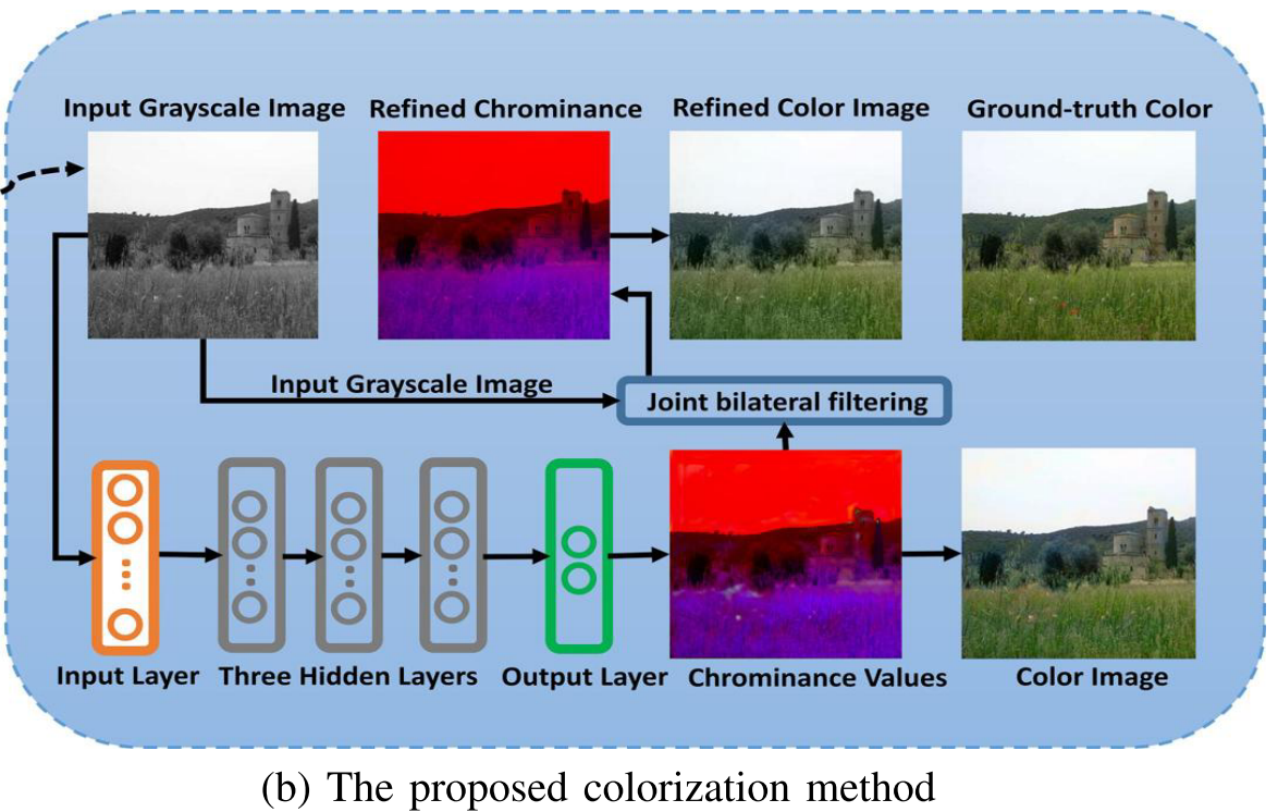
The proposed method has two major steps:

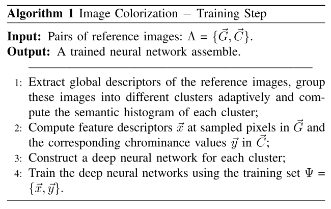
1. Training a neural network assemble using a large set of example reference images
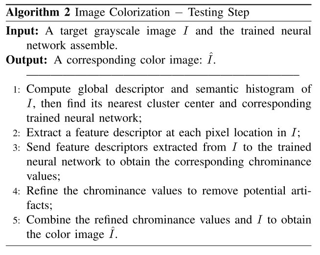
2. Using the learned neural network assemble to colorize a target grayscale image.

Deep Learning Model

Formulation

A deep neural network is a universal approximator that can represent arbitrarily complex continuous functions. Given a set of \(\Lambda={\overrightarrow{G}, \overrightarrow{C}}\), where \(\overrightarrow{G}\) are grayscale images and \(\overrightarrow{C}\) are corresponding color images respectively, our method is based on a premise: there exists a complex gray-to-color mapping function \(\mathcal{F}\) that can map the features extracted at each pixel in \(\overrightarrow{G}\) to the corresponding chrominance values in \(\overrightarrow{C}\). We aim at learning such a mapping function from \(\Lambda\) so that the conversion from a new gray image to color image can be achieved by using \(\mathcal{F}\).

In our model, the YUV color space is employed, since this color space minimizes the correlation between the three coordinate axes of the color space. For a pixel \(p\) in \(\overrightarrow{G}\), the output is simply the U and V channels of the corresponding pixel in \(\overrightarrow{C}\) and the input of \(\mathcal{F}\) is the feature descriptors we compute at pixel \(p\).

We reformulate the gray-to-color mapping function as

where \(x_p\) is the feature descriptor extracted at pixel \(p\) and \(c_p\) are the corresponding chrominance values. \(\Theta\) are the parameters of the mapping function to be learned from the model.

We solve the following least square minimization problem to learn the parameters \(\Theta\):

where \(n\) is the total number of training pixels sampled from \(\Lambda\) and \(\Gamma\) is the function space of the output.

Architecture

In our model, the number of neurons in the input layer is equal to the dimension of the feature descriptor extracted from each pixel location in a grayscale image and the output layer has two neurons which output the U and V channels of the corresponding color value, respectively. Each neuron in the hidden or output layer is connected to all the neurons in the proceeding layer and each connection is associated with a weight.

Let \(o^l_j\) denote the output of the j-th neuron in the l-th layer. \(o^l_j\) can be expressed as follows:

where \(w^l_{ji}\) is the weight of the connection between the \(j^{th}\) neuron in the \(l^{th}\) layer and the \(i^{th}\) neuron in the \((l-1)^{th}\) layer. The output of the neurons in the output layer is just the weighted combination of the outputs of the neurons in the procedding layer.

Feature Descriptor

We separate the adopted features into low-, mid- and high-level features. Let \(x^L_p, x^M_p, x^H_p\) denote different level feature descriptors extracted from a pixel location \(p\), we concatenate these features to construct our feature descriptor \(x_p\).

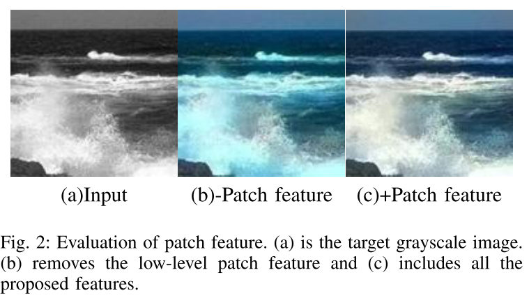
1. Low-level Patch Feature: Intuitively, there exist too many pixels with same luminance but fairly different chrominance in a color image, thus it’s far from being enough to use only the luminance value to represent a pixel. In practice, different pixels typically have different neighbors, using a patch centered at a pixel \(p\) tends to be more robust to distinguish pixel \(p\) from other pixels in a grayscale image. Let \(x^L_p\) denote the array containing the sequential grayscale values in a \(7 \times 7\) patch center at \(p\). Note that our model will be insensitive to the intensity variation within a semantic region when the patch feature is missing

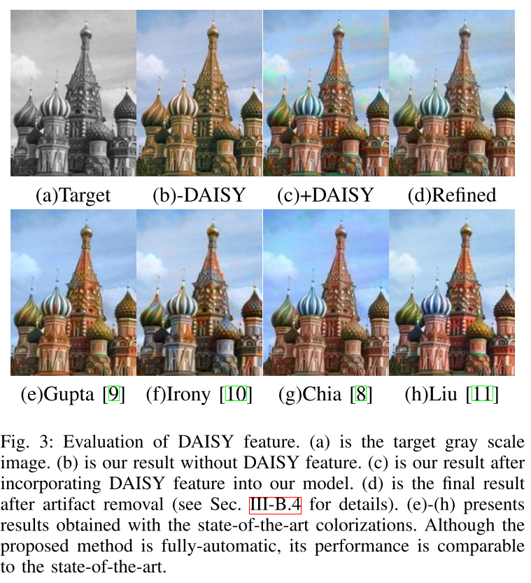
1. Mid-level DAISY Feature: DAISY is a fast local descriptor for dense matching. DAISY can achieve a more accurate discriminative description of a local patch and thus can improve the colorization quality on complex scenarios. A DAISY descriptor is computed and denote as \(x^M_p\). The adoption of DAISY feature in our model leads to a more detailed and accurate colorization result on complex regions. However, DAISY feature is not suitable for matching low-texture regions/objects and thus will reduce the performance around these regions.

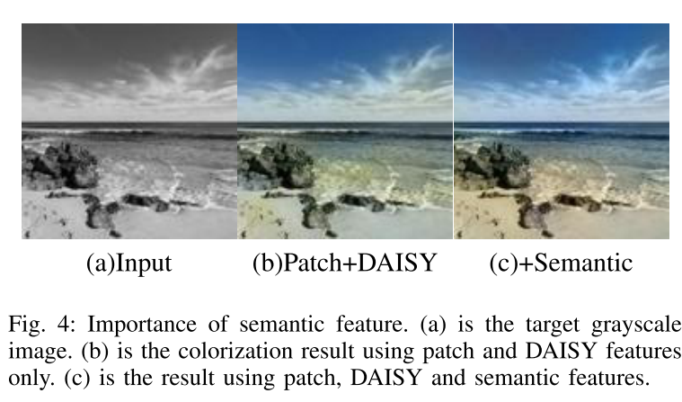
1. High-level Semantic Feature: Considering that the image colorization is typically a semantic- aware process, we extract a semantic feature at each pixel to express its category. We adopt the state-of-art scene parsing algorithm to annotate each pixel with its category label, and obtain a semantic map for the input image. The semantic map is not accurate around region boundaries. As a result, it is smoothed using an efficient edge-preserving filter with the guidance of the original gray scale image. An N-dimension probability vector will be computed at each pixel location, where N is the total number of object categories and each element is the probability that the current pixel belongs to the corresponding category.

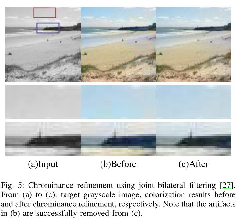
1. Chrominance Refinement: We simply concatenate the two features instead of digging out a better combination. This will result in potential artifacts especially around the low-texture objects (e.g., sky, sea). This is because DAISY is vulnerable to these objects and presents a negative contribution. The artifacts around low-texture regions can be significantly reduced using joint bilateral filtering technique. Our problem is similar, the chrominance values obtained from the trained neural network is noisy (and thus results in visible artifacts) while the target grayscale image is noise-free.

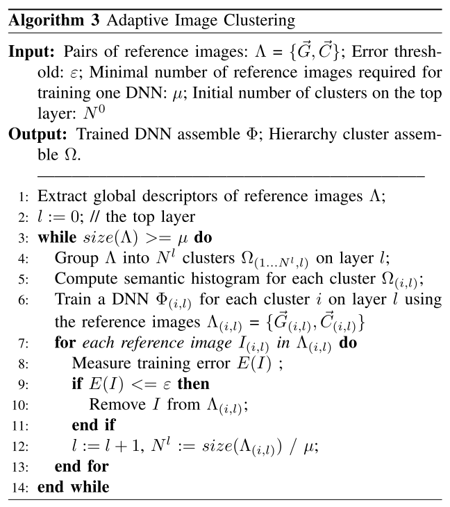
Adaptive Image Clustering

Visible artifacts still appear, especially on the objects with large color variances. One reason is that the receptive field of the DNN is limited on local patch, which causes large training ambiguities especially when large training set is utilized. Intuitively, the global image descriptor is able to reflect the scene category with the robustness to local noise, and there are typically smaller color variances within one scene than mixed scenes. Thus the global information is useful to reduce the matching/training ambiguities and improve the colorization accuracy. We incorporate the global information by an image clustering method. Using adaptive pixel clustering algorithm to trains a regressor assemble to model the light transport, we utilize a similar strategy to split the reference images into different scenes, for each of which a DNN is trained.

The reference images are clustered adaptively on different layers by standard k-means clustering algorithm. After completing the training of DNN for cluster i on layer l, we measure the training error \(E(I_{(i, l)})\) for each reference image \(I_{(i,l)}\) as the negative PSNR computed from the colorization result \(\hat{I}_{(i,l)}\) and the ground truth image.

If \(E(I_{(i, l)})\) is lower than a threshold \(\epsilon\), \(I_{(i,l)}\) will be removed from the reference image set \(\Lambda_{(i,l)}\). As a result, the top layer contains all reference images while the lower layer comprises fewer images.

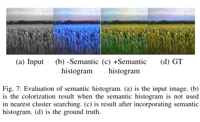
Semantic Histogram: After scene-wise DNNs are trained, a straightforward colorization strategy is to find the nearest cluster for a target image and use the corresponding trained DNN to colorize it. However, it is very likely that the reference images in the searched cluster are globally similar but semantically different from the target images.

Algorithms

It combines three levels of features with increasing receptive field: the raw image patch, DAISY features, and semantic features. These features are concatenated and fed into a three-layer fully connected neural network trained with an L2 loss. Only this last component is optimized; the feature representations are fixed

Let there be color!

Iizuka & Simo-Serra² propose a network that concatenates two separate paths, specializing in global and local features, respectively. They called it Joint Global and Local Model, which means the network is formed by several subcomponents that form a Directed Acyclic Graph (DAG) and contain important discrepancies with widely-used standard models. In particular:

1. can process images of any resolution
2. incorporates global image priors for local predictions
3. can directly transfer the style of an image into the colorization of another.

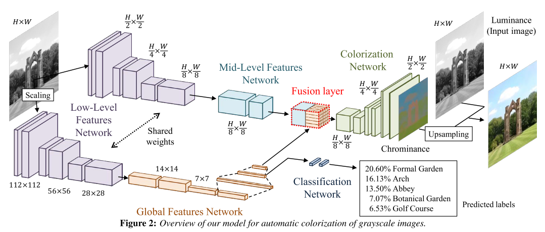
The components are all tightly coupled and trained in an end-to-end fashion. The output of model is the chrominance of the image which is fused with the luminance to form the output image.

Deep Networks

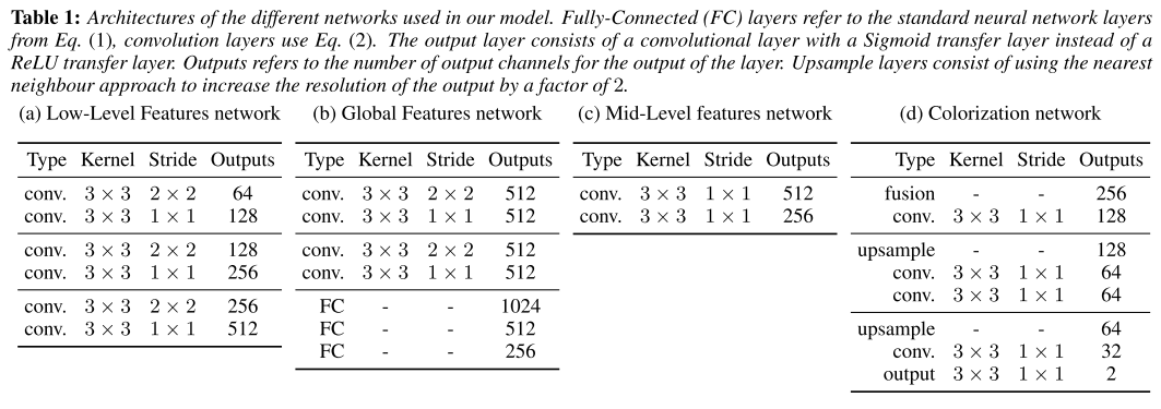
The model use ReLU as activate function, and Sigmoid trasfer function for the color output layer.

Fusing Global and Local Features for Colorization

A 6-layer Convolutional Neural Network obtains low-level features directly from the input image. The convolution filter bank the net- work represents are shared to feed both the global features network and the mid-level features network. Instead of using max-pooling layers to reduce the size of the feature maps, we use convolution layers with increased strides. This is also impor- tant for increasing the spatial support of each layer. If padding is added to the layer, the output is effectively half the size of the input layer. This can be used to replace the max-pooling layers while maintaining performance.

Global Image Features

The global image features are obtained by further processing the low-level features with four convolutional layers followed by three fully-connected layers. This results in a 256-dimensional vector representation of the image. Note that due to the nature of the linear layers in this network, it requires the input of the low-level features network to be of fixed size of 224 × 224 pixels.

Mid-Level Features

The mid-level features are obtained by processing the low-level fea- tures further with two convolutional layers. The output is bottlenecked from the original 512-channel low-level features to 256 channel mid-level features. Note that unlike the global image features, the low-level and mid-level features networks are fully convolutional networks, such that the output is a scaled version of the input. This can be thought of as concatenating the global features with the local features at each spatial location and processing them through a small one-layer network. This effectively combines the global feature and the local features to obtain a new feature map that is, as the mid-level features, a 3D volume. Therefore, the resulting features are independent of any resolution constraints that the global image features might have.

Colorization Network

Once the features are fused, they are processed by a set of convolutions and upsampling layers, the latter which consist of simply upsampling the input by using the nearest neighbour technique so that the output is twice as wide and twice as tall. These layers are alternated until the output is half the size of the original input. The output layer of the colorization network consists of a convolutional layer with a Sigmoid transfer function that outputs the chrominance of the input grayscale image.

In order to train the network, we use the Mean Square Error (MSE) criterion. Given a color image for training, we convert the image to grayscale and CIE Lab colorspace. The input of the model is the grayscale image while the target output is the ab components of the CIE Lab colorspace. The ab components are globally normalized so they lie in the [0, 1] range of the Sigmoid transfer function. We then scale the target output to the size of the output of the colorization network and compute the MSE between the output and target output as the loss. This loss is then back-propagated through all the networks (global features, mid-level features and low-level features) to update all the parameters of the model.

Colorization with Classification

As learning these networks is an non-convex problem, we facilitate the optimization by also training for classification jointly with the colorization. As we train the model using a large-scale dataset for classification ofN classes, we have classification labels available for training. These labels correspond to a global image tag and thus can be used to guide the training of the global image features. We do this by introducing another very small neural network that consists of two fully-connected layers: a hidden layer with 256 outputs and an output layer with as many outputs as the number of classes in the dataset, which is N = 205 in our case. The input of this network is the second to last layer of the global features network with 512 outputs. We train this network using the cross-entropy loss, jointly with the MSE loss for the colorization network. Thus, the global loss of our network becomes:

Optimization and Learning

Note that when the input image size is of a different resolution, while the low-level feature weights are shared, a rescaled image of size 224 × 224 must be used for the global features network. This requires processing both the original image and the rescaled image through the low- level features network, increasing both memory consumption and computation time.

Learning very deep networks such as the one proposed directly from a random initialization is a very challenging task. One of the recent improvements that have made this possible is batch normalization. This has shown to speed up the learning greatly and allow learning of very deep networks from random initializations. We use batch normalization throughout the entire network during training. Once the network is trained, the batch normalization mean and standard deviation can be folded into the weights and the bias of the layer. This allows the network to not perform unnecessary computations during inference.

Therefore, instead of having to experiment and heuristically determine a good learning rate scheduler, we sidestep the problem by using the ADADELTA optimizer. This approach adaptively sets the learning rates for all the network parameters without requiring us to set a global learning rate. We follow the optimization procedure until convergence of the loss.

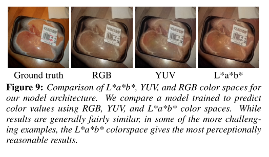
Comparison of Color Spaces

In particular, we compare RGB, YUV and Lab color spaces. In the case of RGB, the output of the model is 3 instead of 2 corresponding to the red, green and blue channels. We train directly using the RGB values; however, for testing, we convert the RGB image to YUV and substitute the input grayscale image as the Y channel of the image. This ensures that the output images of all the models have the same luminance. In the case of YUV and Lab, we output the chrominance and use the luminance of the input image to create the final colorized image. For all different color spaces, we normalize the values to lie in the [0, 1] range of the Sigmoid transfer function of the output layer.In general, results are very similar. However, we do find some cases in which the Lab gives the most reasonable approach in comparison with RGB and YUV. For this reason, we use Lab in our approach.

Baldassarre³ is highly similar to this paper.

Reference

• Previous
  Colorization Insight Scribbled 2
• Next
  Colorization Insight Automatic 2