Header Image: Reddit: Actress Deborah Kerr – promo shot for “From Here To Eternity” (1953)
Evolution
Automatic Colorization
Learning Representations for Automatic Colorization
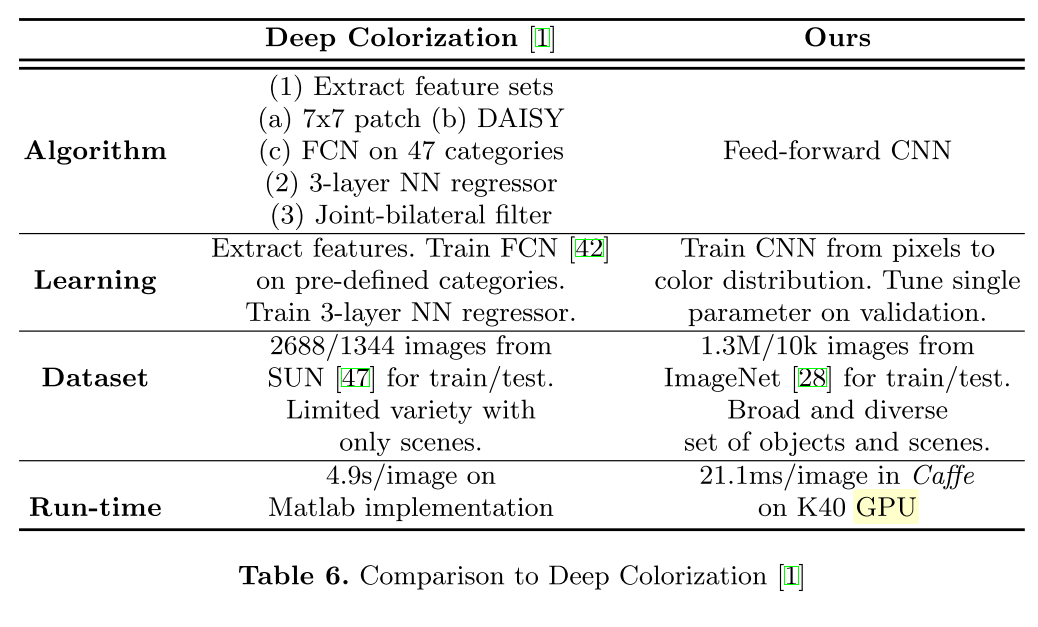
Larsson 1 has developed a fully automatic image colorization system. The system does not rely on hand-crafted features, is trained end-to-end, and treats color prediction as a histogram estimation task rather than as regression.
Method
Given a grayscale image patch \(x \in \mathcal{x} = [0, 1]^{S\times S}, f\) predicts the color \(y \in \mathcal{y}\) of its center pixel. The patch size \(S \times S\) is the receptive field of the colorizer. The output space \(\mathcal{y}\) depends on the choice of color parameterization.
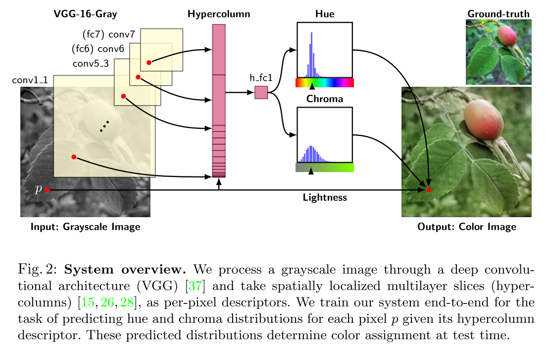
Skip-layer connections, which directly link low- and mid-level features to prediction layers, are an architectural addition beneficial for many image-to-image problems. We use the strategy which extracts per-pixel discriptors by reading localized slices of multiple layers and adopt the recently coined hypercolumn terminology for such slice.
Color Space
We generate training data by converting color images to grayscale according to \(L = \frac{R+B+G}{3}\).
For the representation of color predictions, using RGB is overdetermined, as lightness L is already known. We instead consider output color spaces with L (or a closely related quantity) conveniently appearing as a separate pass-through channel:
- HSL: can be thought of as a color cylinder, with angular coordinate H(hue), radical distance S (saturation), and height L (lightness). The values of S and H are unstable at the bot- tom (black) and top (white) of the cylinder. HSV describes a similar color cylinder which is only unstable at the bottom. However, L is no longer one of the channels. We wish to avoid both instabilities and still retain L as a channel. The solution is a color bicone, where chroma (C) takes the place of saturation. Conversion to HSV is given by \(V=L+\frac{C}{2}, S=\frac{C}{V}\)
- Lab: is designed to be perceptually linear. The color vector (a, b) defines a Euclidean space where the distance to the origin determines chroma.
Loss
At first consideration is L2 regression in Lab:
\[L_{reg}(x,y)=||f(x) - y||\]However, regression targets do not handle multimodal color distributions well. To address this, we instead predict distributions over a set of color bins, a technique also used in:
\[L_{hist}(x,y)=D_{KL}(y||f(x))\]where y describes a histogram over \(K\) bins. The ground-truth histogram y is set as the empirical distribution in a rectangular region of size R around the center pixel. Somewhat surprisingly, our experiments see no benefit to predicting smoothed histograms, so we simply set R = 1. For histogram predictions, the last layer of neural network f is always a softmax.
We bin the Lab axes by evenly spaced Gaussian quantiles (µ = 0, σ = 25). They can be encoded separately for a and b (as marginal distributions), in which case our loss becomes the sum of two separate terms. They can also be encoded as a joint distribution over a and b, in which case we let the quantiles form a 2D grid of bins. In our experiments, we set K = 32 for marginal distributions and K = 16 × 16 for joint. We determined these numbers, along with σ, to offer a good compromise of output fidelity and output complexity.
For hue/chroma, we only consider marginal distributions and bin axes uniformly in [0, 1]. Since hue becomes unstable as chroma approaches zero, we add a sample weight to the hue based on the chroma:
\[L_{hue/chroma}(x,y) = D_{KL}(y_C||f_C(x)) + \lambda_H y_C D_{KL}(y_H||f_H(x))\]where \(y_C\) is the sample pixel’s chroma. We set \(\lambda_H=5\), roughly the inverse expectation of \(y_C\), thus equally weighting hue and chroma.
Inference
For the L2 loss, all that remains is to combine each \(\hat{y}_n\) with the respective lightness and convert to RGB. With histogram predictions, we consider options for inferring a final color:
- Sample: Draw a sample from the histogram. If done per pixel, this may create high-frequency color changes in areas of high-entropy histograms.
- Mode: Take the \(\arg\maxk \hat{y}{n,k}\) as the color. This can create jarring transitions between colors, and is prone to vote splitting for proximal centroids.
- Median: Compute cumulative sum of \(\hat{y}_n\) and use linear interpolation to find the value at the middle bin. Undefined for circular histograms, such as hue.
- Expectation: Sum over the color bin centroids weighted by the histogram.
For Lab output, we achieve the best qualitative and quantitative results using expectations. For hue/chroma, the best results are achieved by taking the median of the chroma. Many objects can appear both with and without chroma, which means \(C = 0\) is a particularly common bin. This mode draws the expectation closer to zero, producing less saturated images. As for hue, since it is circular, we first compute the complex expectation:
\[z=\mathcal{E}_{H~f_h(x)}[H] \triangleq \frac{1}{K}\sum_k [f_h(x)]_k \exp^{i\theta_k},\ \theta_k=2\pi \frac{k + 0.5}{K}\]We then set hue to the argument of z remapped to lie in [0, 1).
In cases where the estimate of the chroma is high and z is close to zero, the instability of the hue can create artifacts. A simple, yet effective, fix is chromatic fading: downweight the chroma if the absolute value of z is too small. We thus re- define the predicted chroma by multiplying it by a factor of \(\max(\eta − 1|z|, 1)\). In our experiments, we set η = 0.03 (obtained via cross-validation).
Neural network architecture and training
The base network is a fully convolutional version of VGG-16 with two changes:
- the classification layer (fc8) is discarded
- the first filter layer (conv1 1) operates on a single intensity channel instead of mean-subtracted RGB.
We extract a hypercolumn descriptor for a pixel by concatenating the features at its spatial location in all layers, from data to conv7 (fc7), resulting in a 12, 417 channel descriptor. We feed this hypercolumn into a fully connected layer with 1024 channels, to which we connect output predictors.
Processing each pixel separately in such manner is quite costly. We instead run an entire image through a single forward pass of VGG-16 and approximate hypercolumns using bilinear interpolation. Extracting batches of only 128 hypercolumn descrip- tors per input image, sampled at random locations, provides sufficient training signal. In the backward pass of stochastic gradient descent, an interpolated hy- percolumn propagates its gradients to the four closest spatial cells in each layer. Locks ensure atomicity of gradient updates, without incurring any performance penalty. This drops training memory for hypercolumns to only 13 MB per image.
We initialize with a version of VGG-16 pretrained on ImageNet, adapting it to grayscale by averaging over color channels in the first layer and rescaling appropriately. Prior to training for colorization, we further fine-tune the network for one epoch on the ImageNet classification task with grayscale input. As the original VGG-16 was trained without batch normalization, scale of responses in internal layers can vary dramatically, presenting a problem for learning atop their hypercolumn concatenation. We use the alternative of balancing hypercolumns so that each layer has roughly unit second moment (E[X2] ≈ 1).
Colorful Image Colorization
Zhang2 has form the problem into model enough of the statistical dependencies between the semantics and the textures of grayscale images and their color versions in order to produce visually compelling results.
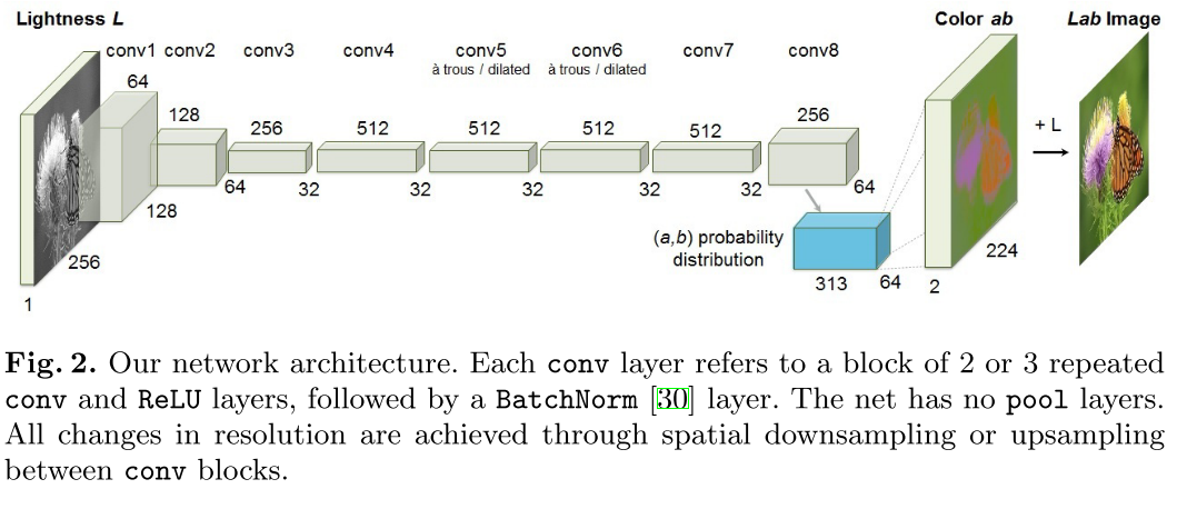
We train a CNN to map from a grayscale input to a distribution over quantized color value outputs using the architecture.
Objective Function
We perform this task in CIE Lab color space. Because distances in this space model perceptual distance is the Euclidean loss:
\[L_2(\hat{Y}, Y) = \frac{1}{2}\sum_{h,w}||Y_{h,w}-\hat{Y}_{h,w}||_2^2\]However, this loss is not robust to the inherent ambiguity and multimodal nature of the colorization problem. If an object can take on a set of distinct ab values, the optimal solution to the Euclidean loss will be the mean of the set. In color prediction, this averaging effect favors grayish, desaturated results. Additionally, if the set of plausible colorizations is non-convex, the solution will in fact be out of the set, giving implausible results.
Instead, we treat the problem as multinomial classification. We quantize the ab output space into bins with grid size 10 and keep the Q = 313 values which are in-gamut. For a given input \(X\), we learn a mapping \(\hat{Z}=\mathcal{G}(X)\) to a probability distribution over possible color \(\hat{Z} \in [0, 1]^{H\times W\times Q}\), where Q is the number of quantized ab values.
To compare predicted \(\hat{Z}\) against ground truth, we define function \(\hat{Z}=\mathcal{H}_{gt}^{-1}(Y)\), which converts ground truth color Y to vector Z, using a soft-encoding scheme.
For soft-enconding scheme:
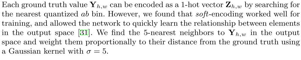
We then use multinomial cross entropy loss:
\[L_{cl}(\hat{Z}, Z) = -\sum_{h,w}v(Z_h, w)\sum_q Z_{h,w,q} \log(\hat{Z}_{h,w,q})\]where \(v()\) is a weighting term that can be used to rebalance the loss based on color-class rarity. Finally, we map probability distribution \(\hat{Z}\) to color values \(\hat{Y}\) with function \(\hat{Y} = \mathcal{H}(\hat{Z})\).
Class Rebalancing
The distribution of ab values in natural images is strongly biased towards val- ues with low ab values, due to the appearance of backgrounds such as clouds, pavement. Observe that the number of pixels in natural images at desaturated values are orders of magnitude higher than for saturated values. Without accounting for this, the loss function is dominated by desaturated ab values. We account for the class-imbalance problem by reweighting the loss of each pixel at train time based on the pixel color rarity. This is asymptotically equivalent to the typical approach of resampling the training space. Each pixel is weighed by factor \(w\in\mathcal{R}^Q\), based on its closest ab bin.
\[v(Z_{h,w}) = w_{q^*},\ where q^*=\arg \max_q Z_{h,w,q}\\ w \propto \large( (1-\lambda) \tilde{p} + \frac{\lambda}{Q}\large)^{-1},\ \mathbb{E}[w] = \sum_q \tilde{p}_qw_q=1\]To obtain smoothed empirical distribution \(p \in \Delta^Q\), we estimate the empirical training set and smooth the distribution with a Gaussian kernel Gσ. We then mix the distribution with a uniform distribution with weight \(\lambda \in [0,1]\), take the reciprocal, and normalize so the weighting factor is 1 on expectation. We found that values of \(\lambda = \frac{1}{2}\) and \(\sigma = 5\) worked well.
Class Probabilities to Point Estimates
We define \(\mathcal{H}\) which maps the predicted distribution \(\hat{Z}\) to point estimate \(\hat{Y}\) in ab space. One choice is to take the mode of the predicted distribution for each pixel. This provides a vibrant but sometimes spatially inconsistent result. On the other hand, taking the mean of the predicted distribution produces spatially consistent but desaturated results. To try to get the best of both worlds, we interpolate by re-adjusting the temperature \(T\) of the softmax distribution, and taking the mean of the result. We draw inspiration from the simulated annealing technique, and thus refer to the operation as taking the annealed-mean of the distribution:
\[\mathcal{H}(Z_{h,w}) =\mathbb{E}[f_T(Z_{h,w})], \ f_T(z)=\frac{\exp(\log(z)/T)}{\sum_q\exp(\log(z_q)/T)}\]Setting \(T=1\) leaves the distribution unchanged, lowering the temperature T produces a more strongly peaked distribution, and setting \(T\rightarrow 0\) results in a 1-hot encoding at the distribution mode. We found that temperature \(T=0.38\) captures the virancy of the mode while maintaining the spatial coherence of the mean.
Our final system \(\mathcal{F}\) is the composition of CNN \(\mathcal{G}\), which produces a predicted distribution over all pixels, and the annealed-mean operation \(\mathcal{H}\), which produces a final prediction.