Header Image: Reddit: Aisin Gioro Puyi, the last emperor of China, as puppet emperor of Manchukuo, wearing the Manzhouguo uniform, circa 1940.

Evolution

Automatic Colorization

Deep Patch-wise Colorization Model for Grayscale Images

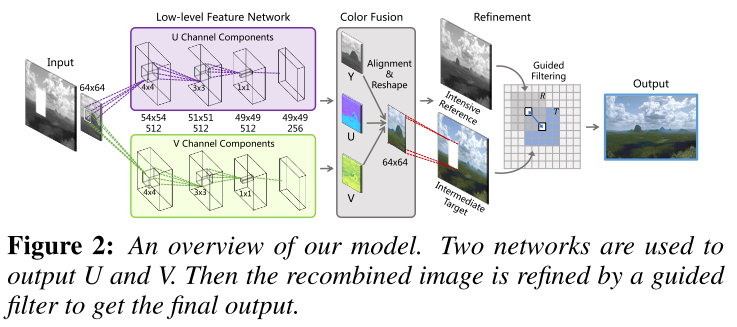
Liang ¹ proposed our model on the basis of vectorized convolutional neu- ral network (VCNN). It mainly consists of three parts: low-level feature network, color fusion and refinement. An overview of our model and its subcomponents are illustrated below.

We find that VCNN can be a bet- ter choice to pursue a faster training speed than traditional CNN. Vectorization refers to the process that transforms the original data structure into a vector representation so that the scalar operators can be converted into a vector implementation.

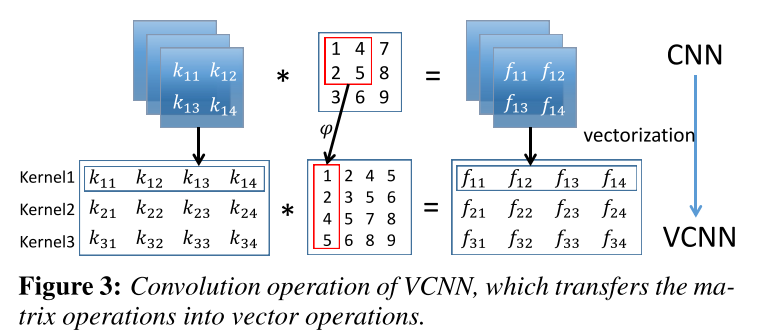
We implement a vectorized colorization network, whose convolu- tion layer realizes a function in this form:

\[[y_i]_i=\sigma([\phi (x)]_i \times [W_i]_i +[b_i]_i)\]

where \(\phi \) referes to the vectorization operator, and operator\([]_i\) is to assemble vectors with index i to form a matrix. This operation is a simplification of extracting matrix from original data or feature map. On the basis of vectorized paradigm, we may reduce the time consumption of the colorization network.

We implement our model in YUV color space. Two networks of the same architecture are used to output U and V respectively.

Network Structure

Deep colorization models could be divided into the following two categories. The local colorization maps color to pixels using the low-, mid- and high-level features while the global colorization incorporates the global features into their models.

In local model, the colorization results of pixels are independent to each other, leading to an unsatisfactory performance. However, it could be a difficult task to evaluate the semantic relationship between neighboring pixels when it comes to global colorization, so the results may not be reasonable.

To take the influence of neighboring pixels into consideration, the output of the network should be smaller than the input. Therefore, we set the output as the center 56x56 area of the input 64x64 patch. Under this setting, our model gets a more compact implementation when compared with the global colorization.

Based on VGG network archi- tecture and the understanding of convolutional network, we finally choose our convolutional kernels as a combination of 11x11, 4x4, 3x3 and 1x1.

Training

The stochastic gradient descent algorithm is used to update the parameters. To pursue a better training performance, we alternately use two loss functions in the process. The first one is MSE. Since this loss function aims to optimize the global error, after 100 iterations, we change out loss function to

\[L(\hat{U}, U)=\min \sum U \log (\hat{U})\]

The loss function focuses on minimizing the local error. It can be a complementary to the previous one for improvement.

To remove the visible artifacts, we use guided filter in the refinement scheme and make full use of the target grayscale image by choosing it as the guidance. The input of the guided filter is the output colorization of neural network, a color image. This scheme can help to reduce artifacts and preserve edges. We set the filter size as 40 and the edge-preserving parameter 1e−4. From the experimental results, most of the artifacts are suppressed after the refinement

I don’t think this paper is very useful.

PIXCOLOR: PIXEL RECURSIVE COLORIZATION

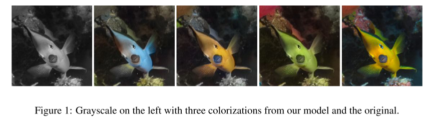
Removing the chromaticity from an image is a subjective operation, thus restoring color to an image is a one-to-many operation.

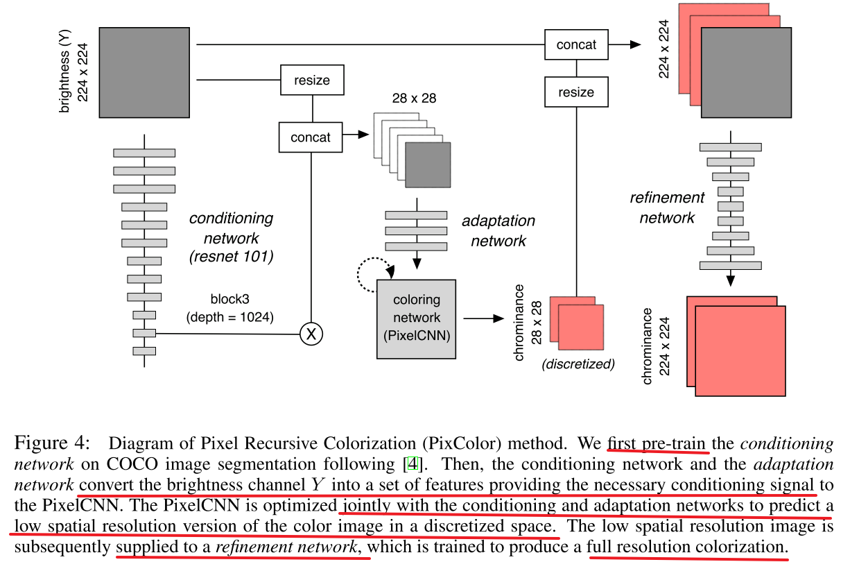
Guadarrama ² propose a new method that employs a PixelCNN probabilistic model to produce a coherent joint distribution over color images given a grayscale input.

PixelCNNs have several advantages over other conditional generative models:

they capture dependencies between the pixels to ensure that colors are selected consistently
the log-likelihood can be computed exactly and training is stable unlike other generative models.

The main disadvantage of PixelCNNs, however, is that they are slow to sample from, due to their inherently sequential (autoregressive) structure.

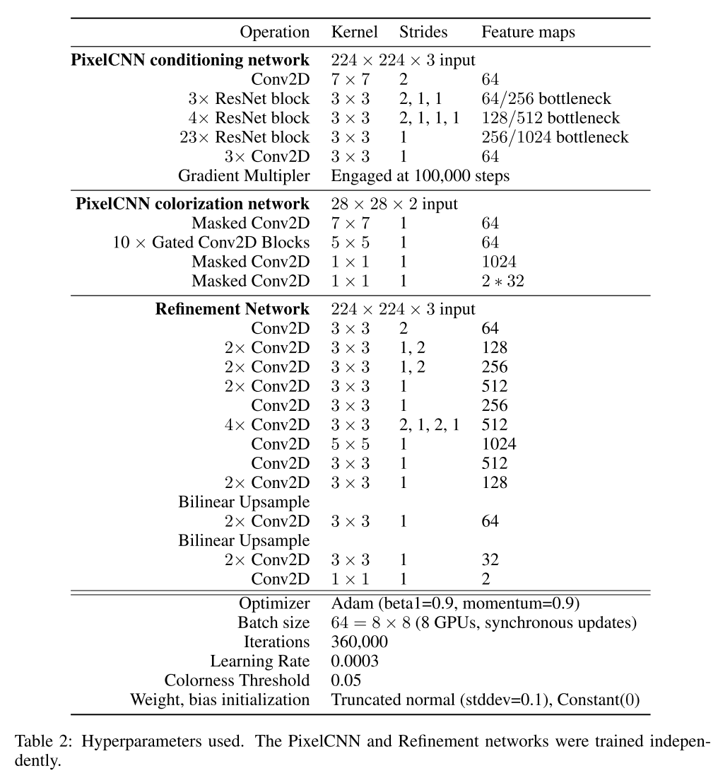
PixelCNN for Low-Resolution Colorization

We use a conditional PixelCNN to produce multiple low resolution color images. That is, we turn colorization into a sequential decision making task, where pixels are colored sequentially, and the color of each pixel is conditioned on the input image and previously colored pixels. Although sampling from a PixelCNN is in general quite slow (since it is inherently sequential), we only need to generate a low-resolution image (28x28), which is reasonably fast. In addition, there are various additional speedup tricks we can use.

We use the YCbCr colorspace, because it is linear, simple and widely used. We discretize the Cb and Cr channels separately into 32 bins. Thus the model has the following the following form:

\[p(y|x)=\prod_i p(y(i, r) | y(1:i-1, :), x)p(y(i,b)|y(i,r), y(1:i-1, :), x)\]

where \(y(i,r\) is the Cr value for pixel i, and \(y(i,b)\) is the Cb value.

We train this model using maximum likelihood, with a cross-entropy loss per pixel. Because of the sequential nature of the model, each prediction is conditioned on previous pixels. During training, we “clamp” all the previous pixels to the ground truth values, and just train the network to predict a single pixel at a time. This can be done efficiently in parallel across pixels.

It is possible to do better by learning how to combine the predicted low resolution color image with the original high resolution grayscale image.

We use an image-to-image CNN which we call the refinement network. It is similar in architecture to the “Let There be Color” but some differences in decoding part. We use bilinear interpolation for upsampling instead of learned upsampling.

The refinement network is trained on a 28x28 downsampling of the ground truth chroma images. The reason we do not train it end-to-end with the PixelCNN is the following: the PixelCNN can generate multiple samples, all of which might be quite far from the true chroma image; if we forced the refinement network to map these to the true RGB image, it might learn to ignore these “irrelevant” color “hints”, and just use the input grayscale image. By contrast, when we train using the true low-resolution chroma images, we force the refinement network to focus its efforts on learning how to combine these “hints” with the edge boundaries which are encoded in the grayscale image.

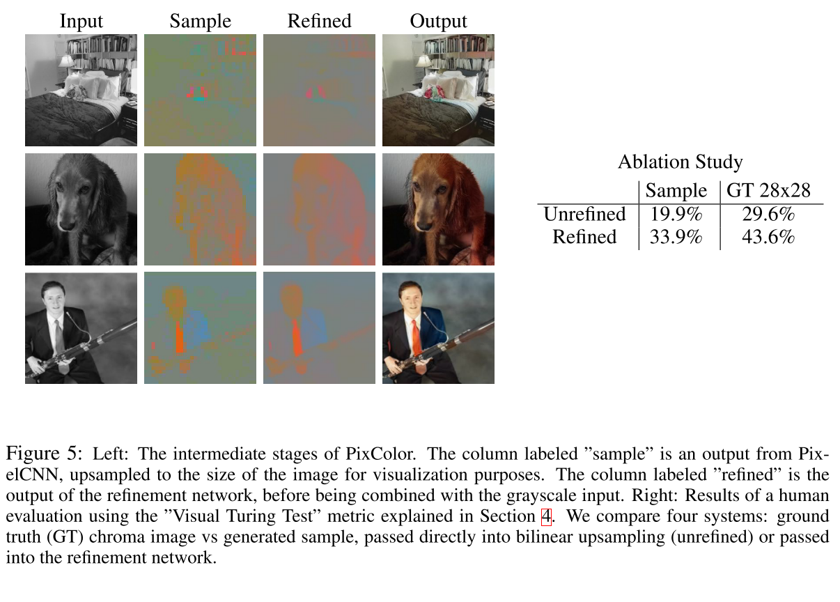
Evaluation Methodology

Since the mapping from gray to color is one-to-many, we cannot evaluate performance by comparing the predicted color image to the ”ground truth” color image in terms of mean squared error or even other perceptual similarity metrics such as SSIM. Instead, we follow the approach and conduct a ”Visual Turing Test” (VTT) using a crowd sourced human raters. In this test, we present two different color versions of an image, one the ground truth and one corresponding to the predicted colors generated by some method. We then ask the rater to pick the image which has the ”true colors”. A method that always produces the ground truth colorization would score 50% by this metric.

Following standard practice, we train on the 1.2M training images from the ILSVRC-CLS dataset, and use 500 images from the “ctest10k” split of the 50k ILSVRC- CLS validation dataset. Each image is shown to 5 different raters. We then compute the fraction of times the generated image is preferred to ground truth; we will call this the ”VTT score” for short.

Model Architecture

Comparison

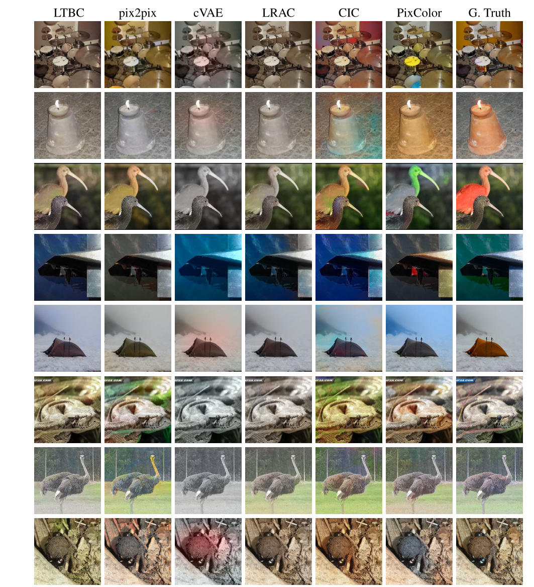
Amelie’w work ³ is very similar to this paper.

Automatic Image Colorization Using Adversarial Training

Shamit ⁴ presented a fully automatic ent-to-end trainable system to colorize grayscale images.

WGAN are models that learn a mapping from noise vector \(z\) to the output image \(y\). The generator network maps the noise \(z\) to output image and critic network approximates the Wasserstein distance between distributions of generated and real images. Conditional WGANs, in contrast, learns a mapping from random noise \(z\) and input image \(x\) to an output image \(y\). The generator does not take noise as input in the proposed approach.

In the proposed model, the last layer of the generator is given as input to a separate classification head to calculate classification loss, which is a softmax cross entropy loss over classification labels. The generator further outputs two tensors, a 64 × 64 × 313 dimensional tensor corresponding to the probability distribution over possible colors for each pixel and a 64 × 64 × 2 dimensional tensor corresponding to a and b channels which is calculated by applying a mapping \(\mathcal{H}\) on the former tensor.

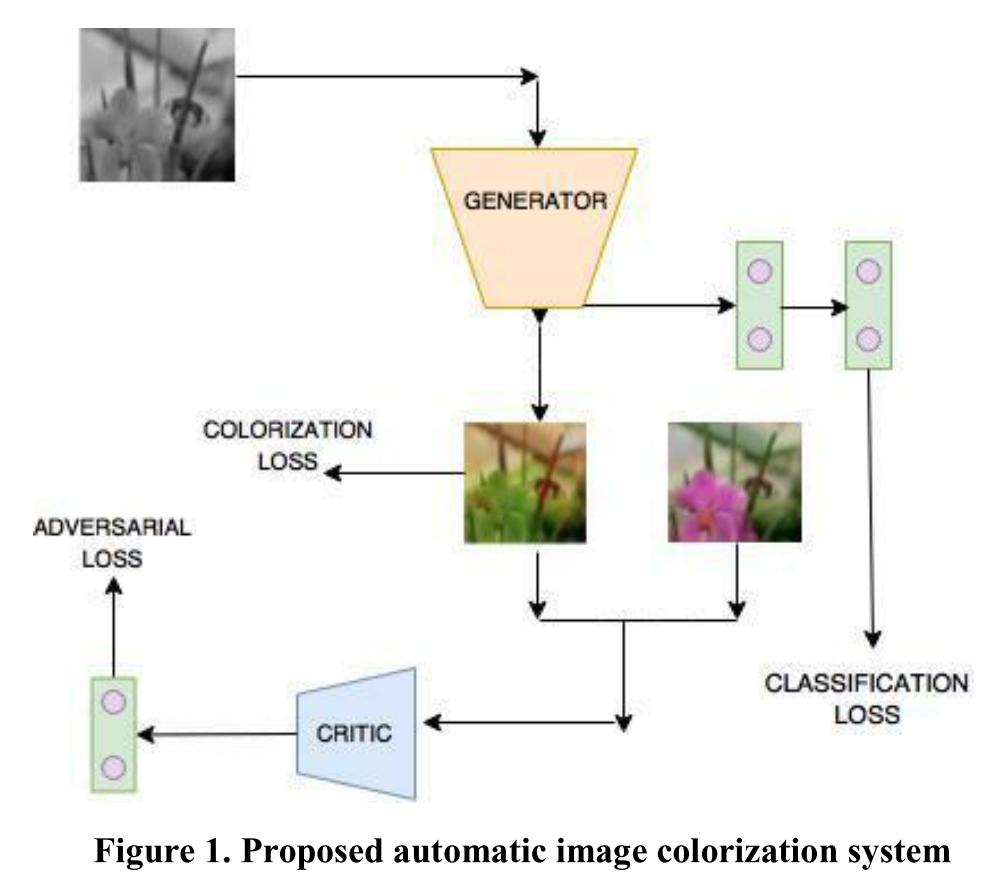
The 64 × 64 × 313 dimensional output tensor is used to calculate colorization loss as explained below. The 64 × 64 × 2 dimensional tensor is concatenated with corresponding lightness channel L and is fed to the critic. The critic also accepts real colored images as input and is trained to approximate Wasserstein distance between the distributions of real and generated images.

Learning Objective

The objective is to learn a mapping function:

\[AB = \mathcal{F}(L), \ AB \in R^{H\times W \times 2}\]

Apart from the adversarial loss learned by WGAN, we propose two additional losses, a colorization loss and a classification loss, in the system. The generator is optimized in order to minimize the following objective:

\[\mathcal{L}_{total} = \lambda_1\mathcal{L}_{co} + \lambda_2\mathcal{L}_{cl} + \lambda_3\mathcal{L}_{g}\]

Adversarial Loss

In WGAN, the generator is optimized to minimize the objective given as:

\[\mathcal{L}_g = -\sum_{L~\mathbb{P}_l}f_w(G_\theta(L)) \\ \mathcal{L}_critic = \sum_{L~\mathbb{P}_l}f_w(G_\theta(L)) - \sum_{C~\mathbb{P}_c}f_w(C)\]

where \(\mathbb{P}_c\) and \(\mathbb{P}_L\) are distributions of colored and graysacle images, \(f\) is the critic network with parameters \(w\) and \(G\) is the generator network with parameters \(\theta\).

Colorization Loss

The ab output space is quantized into bins having grid size 10. Only \(Q = 313\) values, which are in-gamut are kept, out of a total of 400 values. For given input L, a mapping

\[\hat{Z} = \mathcal{G}(L),\ \hat{Z}\in [0,1]^{H\times W\times Q}\]

is learned to a probability distribution over possible colors.

The colorization loss is: \(\mathcal{L}_{co}(\hat{Z}, Z) = -\sum_{h,w}v(Z_{h,w})\sum_qZ_{h,w,q} \log(\hat{Z}_{h,w,q})\)

where \(Z=\mathcal{H}_{gt}^{-1}(Y)\) is a mapping, which uses soft encoding scheme to convert ground-truth color Y to vector Z.

The same as Richard Zhang’s objective Function and Class Rebalancing.

Semantic Label Classification Loss

This loss is a softmax cross-entropy loss over the classification labels. It is applied to the output of classification head, enabling the generator to learn more meaningful features that can distinguish between various classes present in the dataset. The classification loss is:

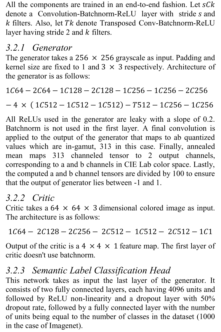
\[\mathcal{L}_{cl}(\hat{C}, C)=-\sum_{classes} C_{class}\log \hat{C}_class\]

Architecture

The system consists of three components: a generator network to produce colored image, a critic network that approximates the Wasserstein distance between distributions of real and generated images and a semantic label classification head.

Highly doubt that this paper is highly borrowed from Richard Zhang’s paper. Just add an GAN architecture.

Reference

Liang X, Su Z, Xiao Y, et al. Deep patch-wise colorization model for grayscale images[M]//SIGGRAPH ASIA 2016 Technical Briefs. 2016: 1-4. ↩
Guadarrama, S., Dahl, R., Bieber, D., Norouzi, M., Shlens, J., & Murphy, K. (2017). Pixcolor: Pixel recursive colorization. British Machine Vision Conference 2017, BMVC 2017, 1–17. https://doi.org/10.5244/c.31.112 ↩
Royer, A., Kolesnikov, A., & Lampert, C. H. (2017). Probabilistic image colorization. British Machine Vision Conference 2017, BMVC 2017, 1–15. https://doi.org/10.5244/c.31.85 ↩
Lal, S., Garg, V., & Verma, O. P. (2017). Automatic image colorization using adversarial training. ACM International Conference Proceeding Series, 84–88. https://doi.org/10.1145/3163080.3163104 ↩

Colorization Insight Automatic 3

More in Deep Learning