Header Image: Reddit: Schoolgirls text messaging in the 40s

Colorization Problem

Color prediction is inherently multimodal – many objects can take on several plausible colorizations. For example, an apple is typically red, green, or yellow, but unlikely to be blue or orange.

Evaluating synthesized images is notoriously difficult. Since our ultimate goal is to make results that are compelling to a human observer, we should introduce a novel way of evaluating colorization results, directly testing their perceptual realism.

Color Space Choosing

YUV

YUV is mostly used in video encoding. Y channel contains the luminance information, which is the content of one image/frame. U and V are chrominance channels, which are contain the color information. The YUV color space is employed, since the color space minimize the correlation between the three coordinates axes of the color space.

YUV and its each components. The image is from Wikipedia.

Cheng ¹, Varga², and Cao³ uses YUV as their training and inference color space.

YCbCr

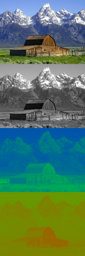
YcbCr is the scaled and offset version of YUV. Cb represents blue component and Cr represents red components. YCbCr colorspace is linear, simple and widely used (e.g., by JPEG).

For example, That the white snow is represented as a middle value in both Cr and Cb; that the brown barn is represented by weak Cb and strong Cr; that the green grass is represented by weak Cb and weak Cr; and that the blue sky is represented by strong Cb and weak Cr. This photo is form the Internet.

Guadarrama ⁴ discretize the Cb and Cr channels separately into 32 bins.

RGB

RGB is the most popular color space in our daily life, it is related to the human eyes perception. But in colorization, none of these channels contains pure image content of pure color information. Only if you put them together, you can see the whole image information.

For the representation of color predictions, using RGB is overdetermined, as lightness L is already known.

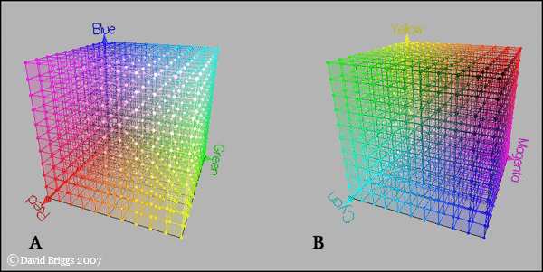
This picture indicate the RGB color space. It is from David Briggs.

Zhu ⁵ use RGB as his training color space.

HSL

Hue-based spaces, such as HSL, can be thought of as a color cylinder, with angular coordinate H (hue), radial distance S (saturation), and height L (lightness). The values of S and H are unstable at the bottom (black) and top (white) of the cylinder. HSV describes a similar color cylinder which is only unstable at the bottom. However, L is no longer one of the channels. He wish to avoid both instabilities and still retain L as a channel. The solution is a color bicone, where chroma (C) takes the place of saturation.

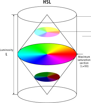
HSL color space. This picture is from Canon Inc.

Larsson ⁶ also used HLS in his experiment.

Lab

CIE Lab is the most usually used color space in colorization. Lab is designed to be perceptually linear. The color vector (a, b) defines a Euclidean space where the distance to the origin determines chroma.

In the L* a* b* color space, L* indicates lightness and a* and b* are chromaticity coordinates. a* and b* are color directions: +a* is the red axis, -a’ is the green axis, +b* is the yellow axis and -b* is the blue axis. Area around the center represents achromatic colors and moving outwards, color saturation increases. The photo is from Konica Minolta.

Apple in Lab. The photo is from Konica Minolta.

Aditya ⁷, Lal ⁸, Baldassarre⁹, Royer¹⁰, Zhang ^{11 12}, Larsson ^{6 13}, Deshpande ¹⁴, Ozbulak¹⁵, Vitoria¹⁶, Nguyen-Quynh¹⁷, Iitsuka¹⁸ and Su¹⁹ all use Lab as their training and inferencing color space.

Comparison on Color Space

Iitsuka¹⁸ has compared the effect of using various color spaces. In particular, they compare RGB, YUV and L* a* b* color spaces.

In the case of RGB, the output of the model is 3 instead of 2 corresponding to the red, green and blue channels. He trained directly using the RGB values; however, for testing, he converted the RGB image to YUV and substitute the input grayscale image as the Y channel of the image. This ensures that the output images of all the models have the same luminance. For all different color spaces, they normalize the values to lie in the [0, 1] range of the Sigmoid transfer function of the output layer.

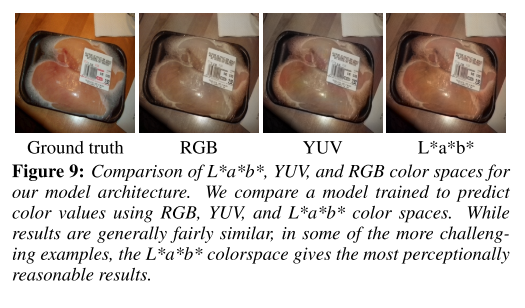
In general, results are very similar. However, they did find some cases in which the L* a* b* gives the most perceptionally reasonable approach in comparison with RGB and YUV.

Neural Network

Most colorization problem can be form into this equation: Given a set of \(\Lambda={\overrightarrow{G}, \overrightarrow{C}}\), where \(\overrightarrow{G}\) are grayscale images and \(\overrightarrow{C}\) are corresponding color images respectively, the method is based on a premise: there exists a complex gray-to-color mapping function \(\mathcal{F}\) that can map the features extracted at each pixel in \(\overrightarrow{G}\) to the corresponding chrominance values in \(\overrightarrow{C}\). We aim at learning such a mapping function from \(\Lambda\) so that the conversion from a new gray image to color image can be achieved by using \(\mathcal{F}\).

non-Generative

Fully Connected

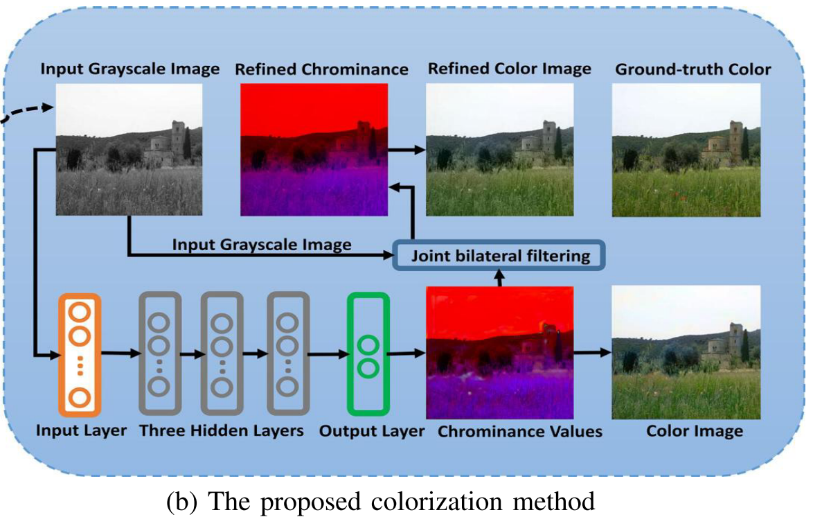
Cheng ¹ maybe the first one propose an automatic colorization method using neural network. In the early stage of deep learning, feature extraction are mostly borrowed from traditional computer vision. The network structure is also based on fully connected layers, which means there are no convolution or other filters. In his model, the number of neurons in the input layer is equal to the dimension of the feature descriptor extracted from each pixel location in a grayscale image and the output layer has two neurons which output the U and V channels of the corresponding color value, respectively. He perceptually set the number of neurons in the hidden layer to half of that in the input layer. Each neuron in the hidden or output layer is connected to all the neurons in the proceeding layer and each connection is associated with a weight.

Feature Descriptor

1. Low-level Patch Feature: the array containing the sequential grayscale values in a 7×7 patch center at pixel p.

2. Mid-level DAISY Feature: DAISY is a fast local descriptor for dense matching.DAISY can achieve a more accurate discriminative description of a local patch and thus can improve the colorization quality on complex scenarios.

3. High-level Semantic Feature: He adopted the state-of-art scene parsing algorithm to annotate each pixel with its category label, and obtain a semantic map for the input image.

End-to-End Convolution + Fully Connected

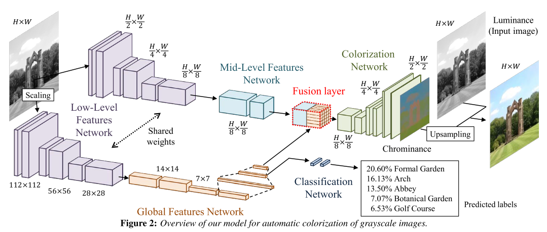
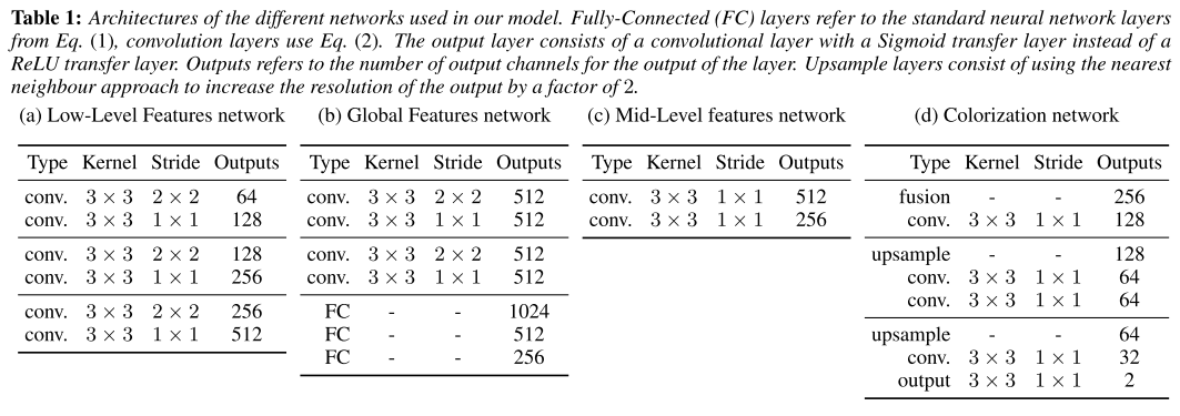
Iizuka & Simo-Serra¹⁸ propose a network that concatenates two separate paths, specializing in global and local features, respectively. They called it Joint Global and Local Model, which means the network is formed by several subcomponents that form a Directed Acyclic Graph (DAG) and contain important discrepancies with widely-used standard models. In particular:

1. can process images of any resolution (which is not unless they discard the global features network)
2. incorporates global image priors for local predictions
3. can directly transfer the style of an image into the colorization of another (End-to-End)

Zhang ¹² implemented a CNN to map from a grayscale input to a distribution over quantized color value outputs using the architecture.

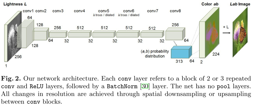
The system is not quite end-to-end trainable, but note that the mapping H operates on each pixel independently, with a single parameter,and can be implemented as part of a feed-forward pass of the CNN. The network was trained from scratch with k-means initialization, using the ADAM solver for approximately 450k iterations.

Fully Convolution

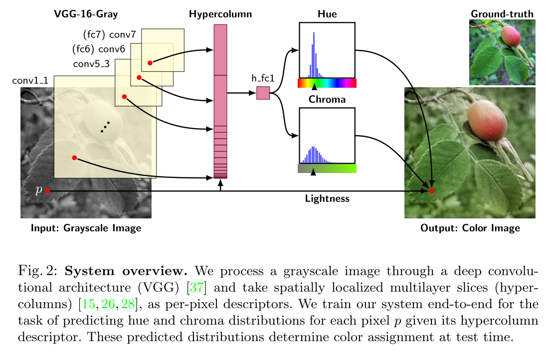
Larsson ⁶ proposed a fully convolution version of VGG-16 with two changes:

1. the classification layer (fc8) is discarded
2. the first filter layer (conv1_1) operates on a single intensity channel instead of mean-subtracted RGB.

He extract a hypercolumn descriptor for a pixel by concatenating the features at its spatial location in all layers, from data to conv7 (fc7), resulting in a 12417 channel descriptor. He fed this hypercolumn into a fully connected layer with 1024 channels (h fc1 in Figure 2), to which he connected output predictors.

Multi-Network

Guadarrama ⁴ propose a new method that employs a PixelCNN probabilistic model to produce a coherent joint distribution over color images given a grayscale input.

That is, he turned colorization into a sequential decision making task, where pixels are colored sequentially, and the color of each pixel is conditioned on the input image and previously colored pixels.

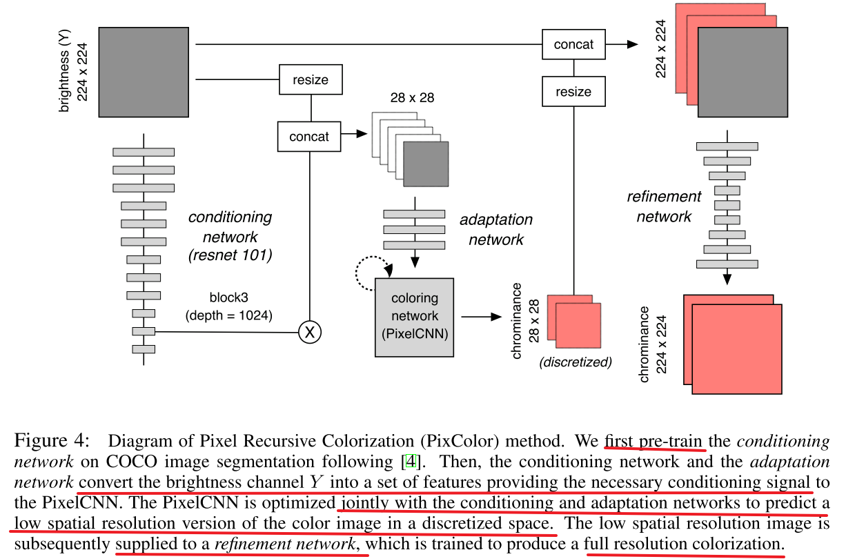
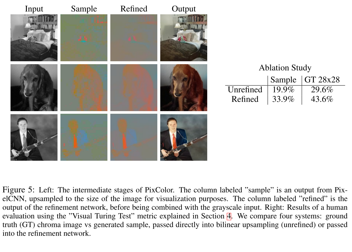
After chrominance of low resolution images, he used bilinear interpolation for upsampling instead of learned upsampling.

The refinement network is trained on a 28x28 downsampling of the ground truth chroma images. The reason he did not train it end-to-end with the PixelCNN is the following: the PixelCNN can generate multiple samples, all of which might be quite far from the true chroma image; if he forced the refinement network to map these to the true RGB image, it might learn to ignore these “irrelevant” color “hints”, and just use the input grayscale image. By contrast, when he trained using the true low-resolution chroma images, he forced the refinement network to focus its efforts on learning how to combine these “hints” with the edge boundaries which are encoded in the grayscale image.

Multi-Module Network

Su proposed both instance colorization network and full-image colorization network. The two networks share the same architecture but different weights.

First, he leveraged an off-the-shelf pre-trained object detector to obtain multiple object bounding boxes \({B_i}^N_{i=1}\) from the grayscale image, where \(N\) is the number of instances. He then generate a set of instance images \({X_i}^N_{i=1}\) by resizing the images cropped from the grayscale image using the detected bounding boxes. Next, he fed each instance image \(X_i\) and input grayscale image \(X\) to the instance colorization network and full-image colorization network, respectively. Finally, he employed a fusion module that fuses all the instance features with the full-image feature at each layer. This step repeats until the last layer and ob- tains the predict color image \(Y\).

He adopt a sequential approach that first trains the full-image network, followed by the instance network, and finally trains the feature fusion module by freezing the above two networks.

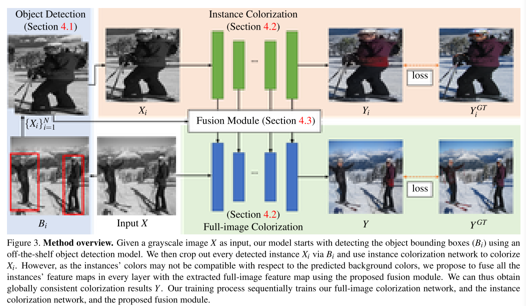
In this work, he adopt the main colorization network introduced in Zhang ²⁰ as our backbones.

The fusion module is shown below

Generative Model

Autoencoder

Zhang ¹¹ propose split-brain autoencoder architecture for unsupervised representation learning.

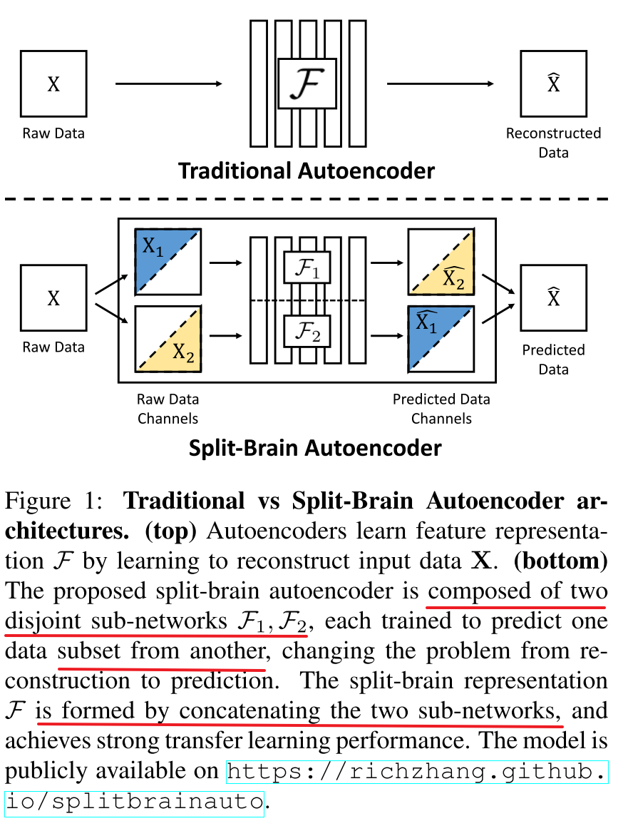
Here is an application on colorization:

VAE (Variation Autoencoder)

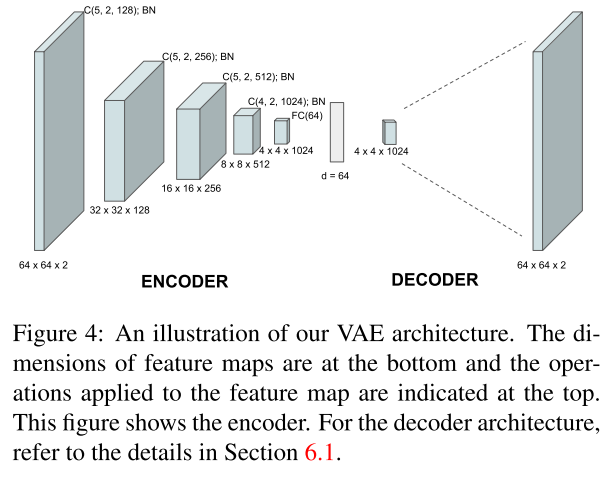
The overall architecture of the network he proposed:

Deshpande’s strategy is to represent \(C\) by its low-dimensional latent variable embedding \(z\). This embedding is learned by a generative model VAE.The encoder network is roughly the mirror of decoder network.

He leveraged a Mixture Density Network (MDN) to learn a multi-modal conditional model \(P(z|G)\). MDN can get a Gaussian Mixture Model (GMM) that generates the low-dimensional embedding. In testing procesdure, he used the VAE decoder to generate the corresponding diverse color fields.

GAN

Single-Module GAN

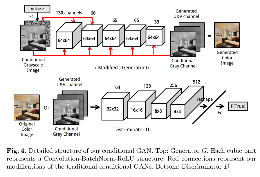
Cao ³ used conditional GANs to generate diverse colorization for a single grayscale image while maintaining their reality. Conditional GAN is a much more suitable framework to handle diverse colorization than other CNNs. Meanwhile, as the discriminator only needs the signal of whether a training instance is real or generated, which is directly provided without any human annotation during the training phase, the task is in an unsupervised learning fashion.

He build a fully convolutional generator and each convolutional layer is splinted by a concatenate layer to continuously render the conditional grayscale information. Additionally, to maintain the spatial information, he set all convo- lution stride to 1 to avoid downsizing data. He also concatenate noise channels to the first half convolutional layers of the generator to attain more diversity in the color image generation process. As the generator G would capture the color distribution, he can alter the colorization result by changing the input noise.

Traditional GANs and conditional GANs receive noise information at the very start layer, during the continuous data transformation through the network, the noise information is attenuated a lot. To overcome this problem and make the colorization results more diversified, he concatenated the noise channel onto the first half of the generator layers (the first three layers in our case).

Multi-Module GAN

Vitoria ¹⁶ proposed the ChromaGAN. It contains three distinct parts. The first two, belonging to the genera- tor, focus on geometrically and semantically generating a color image information (a, b) and classifying its semantic content. The third one belongs to the discriminator network learning to distinguish between real and fake data.

The generator is similar to Iitsuka’s model architecture.

Objective Function

Regression

MSE (Least Squares Minimization/RMSE)

where \(\hat{Y}\) means the predicted result, and \(Y\) is the groundtruth.

However, the results from these previous attempts tend to look desaturated. This loss is not robust to the inherent ambiguity and multimodal nature of the colorization problem. If an object can take on a set of distinct ab values, the optimal solution to the Euclidean loss will be the mean of the set. In color prediction, this averaging effect favors grayish, desaturated results. Additionally, if the set of plausible colorizations is non-convex, the solution will in fact be out of the set, giving implausible results.

Cheng ¹, Iizuka & Simo-Serra¹⁸ used it as the basic colorization loss.

smooth-L1 loss (Huber loss)

Zhang ²⁰ proposed the smooth-L1 loss with δ = 1:

The original huber loss is:

When \(\delta\) approching 0, huber loss will be MAE; Otherwise, huber loss will be MSE.

KL Divergence

Larsson ⁶ predict distributions over a set of color bins, using

where y describes a histogram over \(K\) bins. The ground-truth histogram y is set as the empirical distribution in a rectangular region of size R around the center pixel.We simply set R = 1. For histogram predictions, the last layer of neural network f is always a softmax.

He bin the Lab axes by evenly spaced Gaussian quantiles (µ = 0, σ = 25). They can be encoded separately for a and b (as marginal distributions), in which case our loss becomes the sum of two separate terms. They can also be encoded as a joint distribution over a and b, in which case he let the quantiles form a 2D grid of bins. In our experiments, he set K = 32 for marginal distributions and K = 16 × 16 for joint. He determined these numbers, along with σ, to offer a good compromise of output fidelity and output complexity.

Classification

Corss-Entropy loss

Iizuka & Simo-Serra¹⁸ finds that the MSE criterion makes obvious mistake due to not properly learning the global context of the image. So they facilitate the optimization by also training for classification jointly with the colorization. Classification labels correspond to a global image tag and thus can be used to train for global image feature. They introduced the cross-entropy loss, jointly with the MSE loss for the colorization network.

Thus, the global loss becomes:

Multinomial Classification

Zhang ¹² treated the colorization problem as multinomial classification. Instead, he treat the problem as multinomial classification. He quantized the ab output space into bins with grid size 10 and keep the Q = 313 values which are in-gamut. For a given input \(X\), he learned a mapping \(\hat{Z}=\mathcal{G}(X)\) to a probability distribution over possible color \(\hat{Z} \in [0, 1]^{H\times W\times Q}\), where Q is the number of quantized ab values.

To compare predicted \(\hat{Z}\) against ground truth, we define function \(\hat{Z}=\mathcal{H}_{gt}^{-1}(Y)\), which converts ground truth color Y to vector Z, using a soft-encoding scheme.

For soft-enconding scheme:

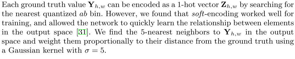
He then used multinomial cross entropy loss:

where \(v(\cdot)\) is a weighting term that can be used to rebalance the loss based on color-class rarity. Finally, he mapped probability distribution \(\hat{Z}\) to color values \(\hat{Y}\) with function \(\hat{Y} = \mathcal{H}(\hat{Z})\).

He accounted for the class imbalance problem by re-weighting the loss of each pixel at train time based on the pixel color rarity. Each pixel is weighed by factor \(w\in R^Q\), based on its closest ab bin.

To obtain smoothed empirical distribution \(p \in \Delta^Q\), he estimated the empirical training set and smooth the distribution with a Gaussian kernel \(G\sigma \). He then mix the distribution with a uniform distribution with weight \(\lambda \in [0,1]\), take the reciprocal, and normalize so the weighting factor is 1 on expectation. He found that values of \(\lambda = \frac{1}{2}\) and \(\sigma = 5\) worked well.

He defined \(\mathcal(H)\), which maps the predicted distribution \(\hat(Z)\) to point estimate \(\hat(Y)\) in ab space. One choice is to take the mode of the predicted distribution for each pixel. On the other hand, takeing the mean of the predicted distribution, but desaturated result. To try to get the best of both worlds, he interpolated by re-adjusting the temperature \(T\) of the softmax distribution, and taking the mean of the result.

He found that temperature \(T=0.38\) captures the virancy of the mode while maintaining the spatial coherence of the mean.

Pixel CNN Loss

Guadarrama ⁴ discretized the Cb and Cr channels separately into 32 bins. Thus the model has the following the following form:

where \(y(i,r)\) is the Cr value for pixel i, and \(y(i,b)\) is the Cb value.

He trained this model using maximum likelihood, with a cross-entropy loss per pixel. Because of the sequential nature of the model, each prediction is conditioned on previous pixels.

VAE loss

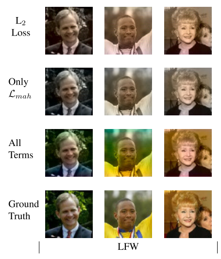
Decoder loss

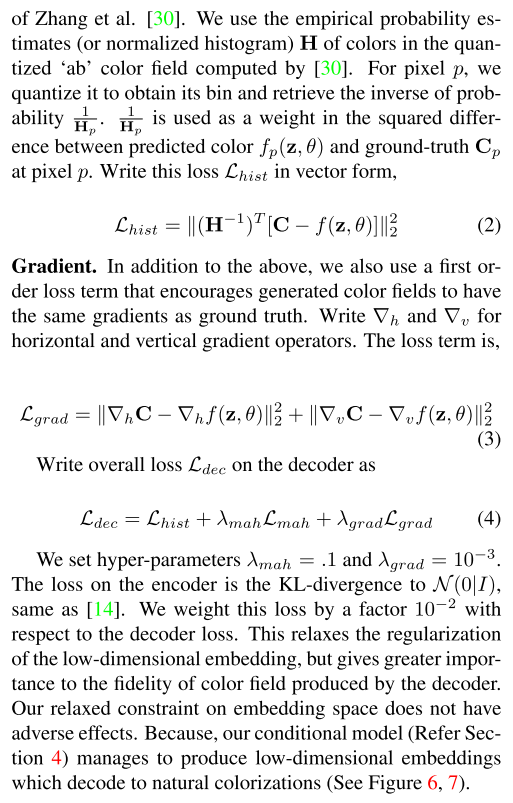
MDN loss

Loss comparison：

GAN loss

Pure GAN loss

The objective of a GAN can be expressed as

Conditional GAN loss

while the objective of a conditional GAN is

where G tries to minimize this objective against an adversarial D that tries to maximize it

Without z, the generator could still learn a mapping from y to x, but would produce deterministic outputs.

GAN loss combination

Vitoria ¹⁶ proposed ChromaGAN which contains multipal loss. The generator model combines two different modules. So there will be \(G_{\theta 1}^1, G_{\theta 2}^2\) Its objective loss is defined by:

The first term denotes the color error loss, using Euclidean Loss.

The last item is

denotes the class distribution loss, where \(\mathbb{P}_{rg}\) denotes the distribution of grayscale input images, and \(y_v\) the output distribution vector of a pre-trained VGG-16 model applied to the grayscale image.

Finally, \(L_g\) denotes the WGAN loss which consists of an adversarial Wasserstein GAN loss. Leverage the WGAN instead of other GAN losses favours nice properties such as avoiding vanishing gradients and mode collapse, and achieves more stable training.

where \(\mathbb{P}G{\theta 1}^1\) is the model distribution of \(G_{\theta 1}^1(L)\), with \(L~\mathbb{P}{rg}\). \(\mathbb{P}{\tilde{I}}\) is implicitly defined sampling uniformly along striaight line between pairs of points sampled from the data distribution \(\mathbb{P}_r\) and the generator distribution

Evaluation Methods

Objective Evaluation

Raw Accuracy

As a low-level test, Richard ¹² computed the percentage of predicted pixel colors within a thresholded L2 distance of the ground truth in ab color space. But note that this AuC metric measures raw prediction accuracy, whereas our method aims for plausibility. So this evaluation method may not quite fit for colorization task.

PSNR

Peak signal-to-noise ratio, often abbreviated PSNR, is an engineering term for the ratio between the maximum possible power of a signal and the power of corrupting noise that affects the fidelity of its representation.

PSNR is most easily defined via MSE, so most MSE loss model are using PSNR as their evaluation index. But in fact, PSNR is not the suitable index for colorization. Due to the multimodel characteristic of colorization output, PSNR can only compare to the groudtruth, but not the perceptual level.

SSIM Family

The structural similarity (SSIM) index is a method for predicting the perceived quality of images. SSIM is designed to improve on traditional methods such as peak signal-to-noise ratio (PSNR) and mean squared error (MSE).

Since the mapping from gray to color is one-to-many, we cannot evaluate performance by comparing the predicted color image to the ”ground truth” color image in terms of perceptual similarity metrics such as SSIM.

Semantic Interpretability (VGG classification)

Richard ¹² tested this by feeding our fake colorized images to a VGG network that was trained to predict ImageNet classes from real color photos. Using an off-the-shelf classifier to assess the realism of synthesized data.

Subjective Evaluation

Perceptual Realism (User Study)

Iizuka & Simo-Serra¹⁸ has performed a user study asking the question “Does this image look natural to you?” to evaluate the naturalness of the ground- truth validation images, the results of our baseline, and the results of our model.

Richard ¹² ran a real vs. fake two-alternative forced choice experiment on Amazon Mechanical Turk (AMT).

Reference

• Previous
  Colorization Insight Automatic 4
• Next
  How to write a good Survey Review