Deep learning in bioinformatics: introduction, application, and perspective in big data era
Abstract
In this review, we provide both the exoteric introduction of deep learning, and concrete examples and implementations of its representative applications in bioinformatics. We start from the recent achievements of deep learning in the bioinformatics field, pointing out the problems which are suitable to use deep learning.
Introduction
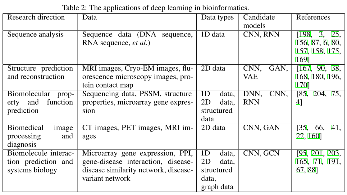
Deep learning has clearly demonstrated its power in promoting the bioinformatics field, including sequence analysis, structure prediction and reconstruction, biomolecular property and function prediction, biomedical image processing and diagnosis, and biomolecule interaction prediction and systems biology.
The core reason for deep learning’s success in bioinformatics is the data. The enormous amount of data being generated in the biological field.
In particular, deep learning has shown its superiority in dealing with the following biological data types.
- Firstly, deep learning has been successful in handling sequence data, such as DNA sequences. Trained with backpropagation and stochastic gradient descent, deep learning is expert in detecting and identifying the known and previously unknown motifs, patterns and domains hidden in the sequence data. Recurrent neural networks and convolutional neural networks with 1D filters are suitable for dealing with this kind of data.
- Secondly, deep learning is especially powerful in processing 2D and tensor-like data, such as biomedical images and gene expression profile. With the help of convolutional layers and pooling layers, these networks can systematically examine the patterns hidden in the original map in different scales and map the original input to an automatically determined hidden space, where the high level representation is very informative and suitable for supervised learning.
- Thirdly, deep learning can also be used to deal with graph data. The core task of handling networks is to perform node embedding, which can be used to perform downstream analysis, such as node classification, interaction prediction and community detection. Compared to shallow embedding, deep learning based embedding, which aggregates the information for the node neighbors in a tree manner, has less parameters and is able to incorporate domain knowledge.
From Shallow Neural Networks to Deep Learning
Shallow Neural Networks and their Components
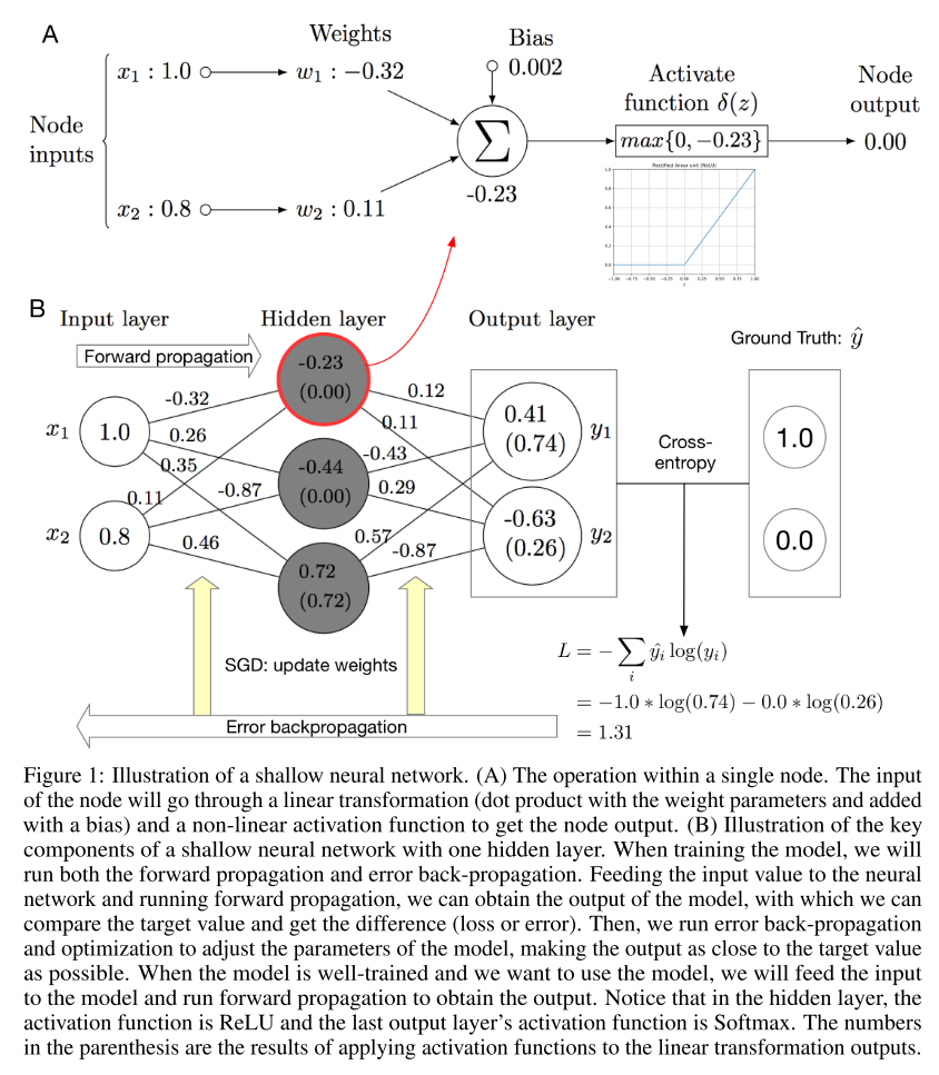
Fig. 1 shows the major components of a shallow neural network. In general, the whole network is a mapping function. Each subnetwork is also a mapping function. By aggregating multiple building block functions into one layer and stacking two layers, we obtain the network shown in Fig. 1 (B), which is capable of expressing a nonlinear mapping function with a relatively high complexity. By comparing the output of the model and the ground truth label, we can compute the difference between the two with a certain loss function. Using the gradient chain rule, we can back-propagate the loss to each parameter and update the parameter with certain update rule. We will run the above steps iteratively (except for the random initialization) until the model converges or reaches a pre-defined number of iterations.
From the above description, we can conclude that multiple factors in different scales can influence the model’s performance.
- The choice of the activation function can influence the model’s capacity and the optimization steps greatly
- How many blocks we want to aggregate in one layer. The more nodes we put into the neural network, the higher complexity the model will have.
- We need to determine which loss function we want to use and which optimizer we prefer.
There are two drawbacks of shallow neural networks:
- The number of parameters is enormous. Such a large number of parameters can cause serious overfitting issue and slow down the training and testing process.
- The shallow neural network considers each input feature independently, ignoring the correlation between input features, which is actually common in biological data.
Legendary deep learning architectures: CNN and RNN
CNN
The convolution neural network has been proposed, which has two characteristics:
- local connectivity
- weight sharing
After necessary pre-processing, such as denoising and normalization, the data vector will go through several (N) convolutional layers and pooling layers, after which the length of the vector becomes shorter but the number of channels increases. After the last pooling layer, the multi-channel vector will be flatten into a single-channel long vector.
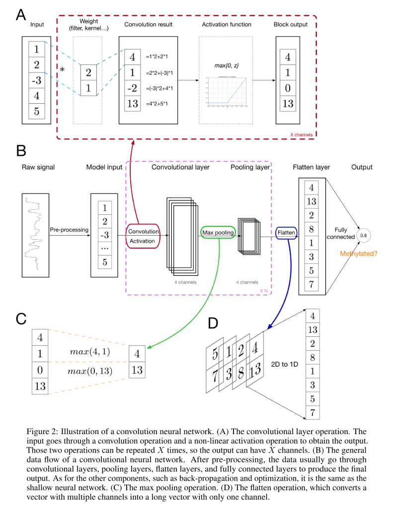
Fig. 2 (A) shows the convolutional layer within CNN in more details. The weight vector slides across the input vector, performing inner product at each position and obtaining the convolution result. Then, an activation function is applied to the convolution result elementwisely, resulting in the convolutional layer output. In convolutional layers, different parts of the input vector share the same weight vector when performing the sliding inner product (convolution), which is the weight-sharing property. Under this weight-sharing and local connectivity setting, we can find that the weight vector serves as a pattern or motif finder, which satisfies our original motivation of introducing this architecture.
Fig. 2 (C) shows the max pooling operation. In the max pooling layer, each element of the output is the maximum of the corresponding region in the layer input. This pooling layer enables the network to capture higher level and long range property of the input vector, such as the long range interaction between the bases within the corresponding DNA sequences of the input signals.
Fig. 2 (D) shows the flatten layer. This operation is straightforward, just concatenating the input vectors with multiple channels into a long vector with only one channel to enable the downstream fully connected layer operation.
RNN
In addition to the spatial dependency within the input, we also need to consider the temporal or order dependency in the input. Recurrent neural networks are specifically designed to exploit the temporal relationship within a sequential input.
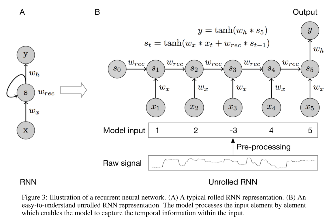
The basic structure of a recurrent neural network is shown in Fig. 3. The hidden recurrent cell has an initial state, which is denoted as \(s_0\) and can be initialized randomly. After taking the first value, the recurrent node is updated, considering the previous state \(s0\) and \(x_1\). When the second value comes in, the node state is updated to \(s_2\) with the same rule. We repeat the above process until we consider all the elements. Then the node information will be fed forward to make predictions. Notice that \(w_x\) and \(w_{rec}\) are shared among all the time steps or positions for that specific hidden recurrent node. Usually, one single recurrent node is not enough to capture all the temporal information.
SOTA Deep Architectures
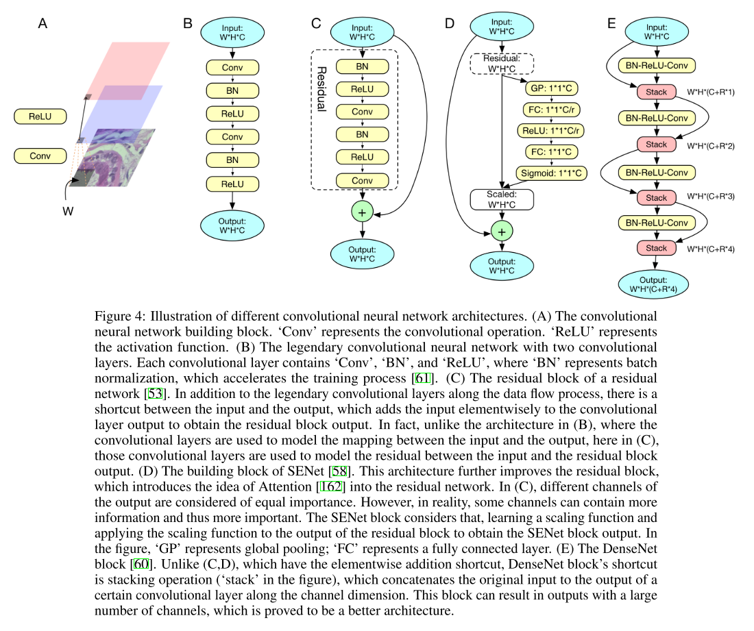
In Fig. 4, we exhibit some typical CNN architectures to deal with 2D image data, showing the evolving of convolutional neural networks. In general, the more advanced CNN architectures allow people to stack more layers, with the hope to extract more useful hidden informations from the input data at the expense of more computational resources. For recurrent neural networks, the more advanced architectures help people deal with the gradient vanishing or explosion issue and accelerate the execution of RNN.
Graph Neural Network
Unlike the sequence and image data, network data are irregular: a node can have arbitrary connection with other nodes. The network information is very important for bioinformatics analysis, because the topological information and the interaction information often have a clear biological meaning, which is a helpful feature for perform classification or prediction. When we deal with the network data, the primary task is to extract and encode the topological and connectivity information from the network, combining that information with the internal property of the node.
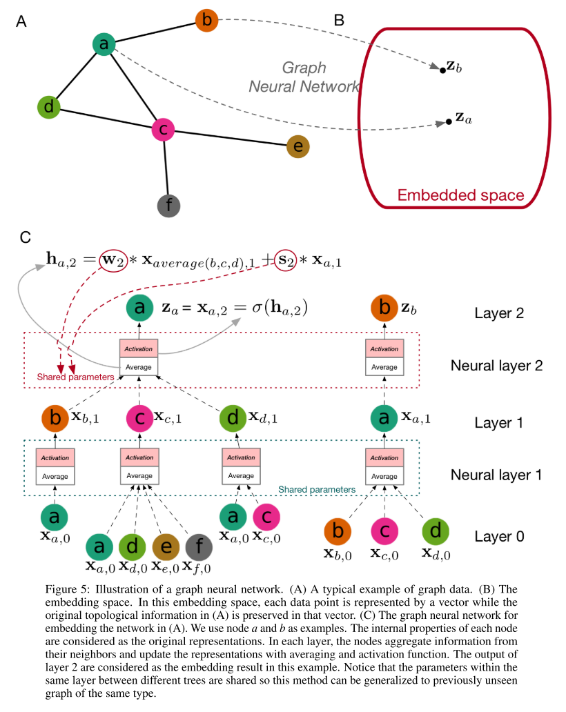
Fig. 5 (A) shows a protein-protein interaction network and each node in the network represents a protein. In addition to the interaction information, each protein has some internal properties, such as the sequence information and the structure information.
What we need to do is to encode the protein in the network in a way that we consider both the network information and the properties, which is known as an embedding problem. In other words, we embed the network data into a regular space, as shown in Fig. 5 (B), where the original topological information is preserved.
For an embedding problem, the most important thing is to aggregate information from a node’s neighbor nodes. Graph convolutional neural networks (GCN), shown in Fig. 5 (C) are designed for such a purpose. Suppose we consider a graph neural network with two layers. For each node, we construct a neighbor tree based on the network. Then we can consider layer 0 as the neural network inputs, which can be the proteins’ internal property encoding in our setting. Then, node a’s neighbors aggregate information from their neighbors, followed by averaging and activating, to obtain their level 1 representation. After that, node a collects information from its neighbors’ level 1 representation to obtain its level 2 representation, which is the neural networks’ output embedding result in this example.
the information collection (average) rule is:
\[\textbf{h}_{a,2} = \textbf{w}_2 \times \textbf{x}_{average(b,c,d), 1} + \textbf{s}_2 \times \textbf{x}_{a, 1}\]where \(x_{average(b,c,d), 1}\) is the average of node \(b, c, d\)’s level 1 embedding, \(x_{a, 1}\) is node a’s level 1 embedding, and \(\textbf{w}_2\) and \(\textbf{s}_2\) are the trainable parameters.
To obtain the level 2 embedding, we apply an activation function to the average result: \(x_{a, 2}=\sigma (h_{a, 2}\).
Notice that between different nodes, the weights within the same neural layer are shared, which means the graph neural network can be generalized to previously unseen network of the same type.
Generative Models: GAN and VAE
GAN and VAE can be useful for biological and biomedical image processing and protein or drug design. The generative models belong to unsupervised learning, which cares more about the intrinsic properties of the data. With generative models, we want to learn the data distribution and generate new data points with some variations.
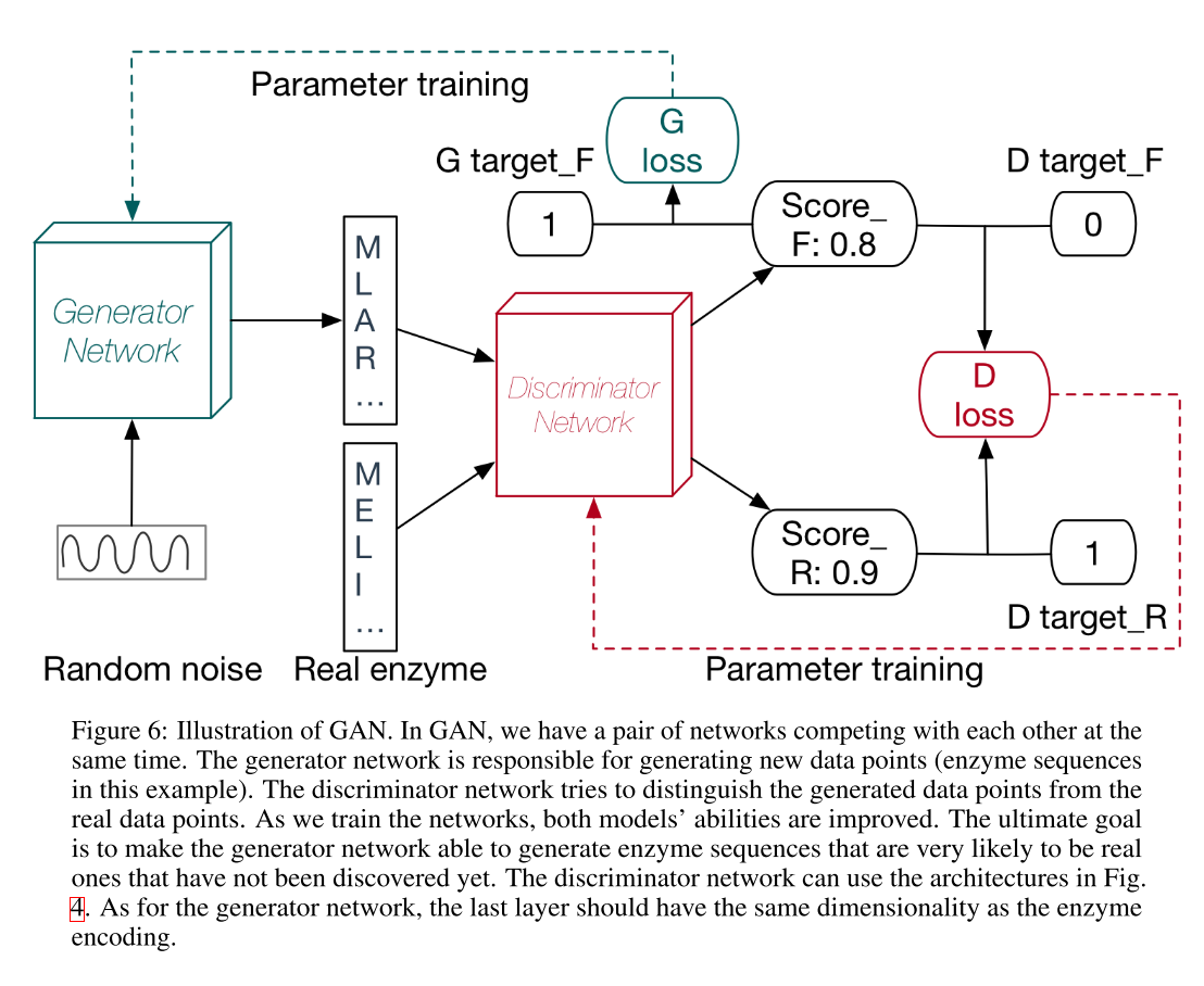
As shown in Fig. 6, instead of training only one neural network, GAN trains a pair of networks which compete with each other. The generator network is the final productive neural network which can produce new data samples while the discriminator network distinguishes the designed enzyme sequences from the real ones to push the generator network to produce protein sequences that are more likely to be enzyme sequences instead of some random sequences. For the generator network, the last layer needs to be redesigned to match the dimensionality of an enzyme sequence encoding.
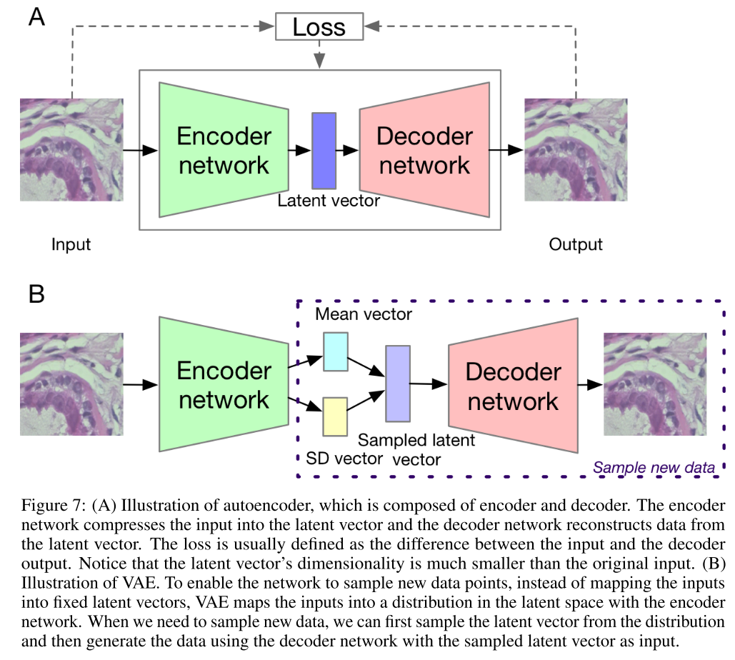
The variational autoencoder is shown in Fig. 7. The autoencoder is usually used to encode high dimensional input data, such as an image, into a much lower dimensional representation, which can store the latent information of the data distribution. It contains two parts, the encoder network and the decoder network. The encoder network can transform the input data into a latent vector and the decoder network can reconstruct the data from the latent vector with the hope that the reconstructed image is as close to the original input as possible. Autoencoder is very convenient for dimensionality reduction. However, we cannot use it to generate new data which are not in the original input. Variational antoencoder overcomes the bottleneck by making a slight change to the latent space. Instead of mapping the input data to one exact latent vector, we map the data into a low dimensional data distribution.
Applications of Deep Learning in Bioinformatics
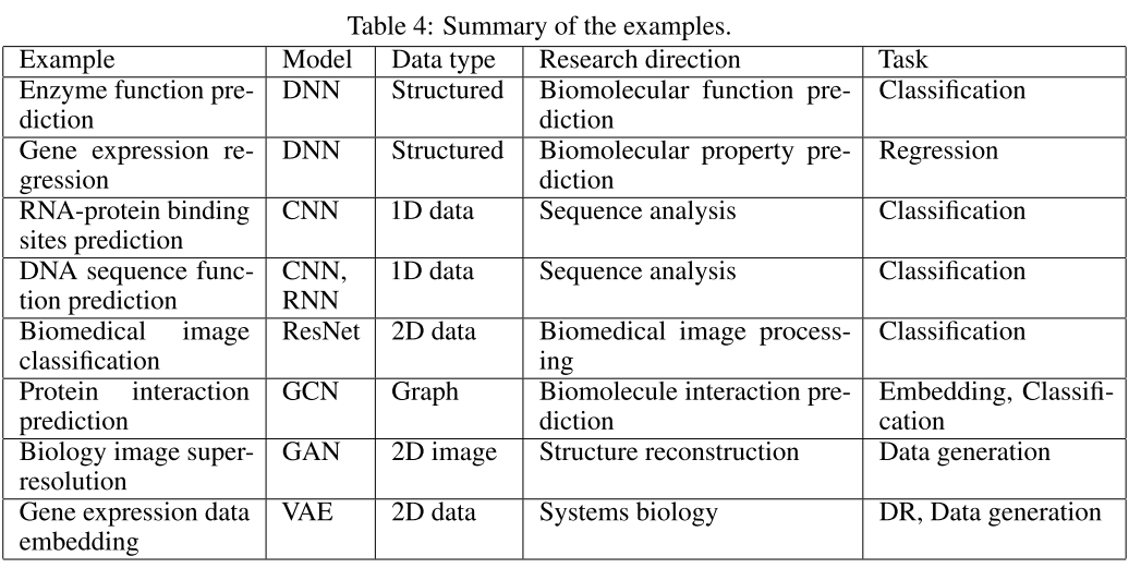
The examples are carefully selected, typical examples of applying deep learning methods into important bioinformatic problems, which can reflect all of the above discussed research directions, models, data types, and tasks, as summarized in Table 4.
Identifying Enzymes Using Multi-Layer Neural Network
Accurately identifying enzymes and predicting their function can benefit various fields, such as biomedical diagnosis and industrial bio-production. In this example, we show how to identify enzyme sequences based on sequence information using deep learning based methods.
So before building the deep learning model, we need to first encode the protein sequences into numbers. In this example, we use a sparse way to encode the protein sequences, the functional domain encoding. For each protein sequence, we use HMMER to search it against the protein functional domain database, Pfam. If a certain functional domain is hit, we encode that domain as 1, otherwise 0. Since Pfam has 16306 functional domains, we have a 16306D vector, composed of 0s and 1s, to encode each protein sequence.
As for the dataset, we use the NEW dataset from the author’s previous work, which contains 22168 enzyme sequences and 22168 non-enzyme protein sequences, whose sequence similarity is under 40% within each class.
The paper claimed that:
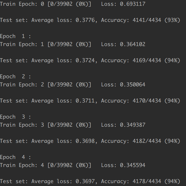
In our implementation, … We use ReLU as the activation function, cross-entropy loss as the loss function, and Adam as the optimizer. We utilize dropout, batch normalization and weight decay to prevent overfitting. With the help of Keras, we build and train the model in 10 lines. Training the model on a Titan X for 2 minutes, we can reach around 94.5% accuracy, which is very close to the state-of-the-art performance. Since bimolecular function prediction and annotation is one of the main research directions of bioinformatics, researchers can easily adopt this example and develop the applications for their own problems.
The network architecture of their implemetation is like:
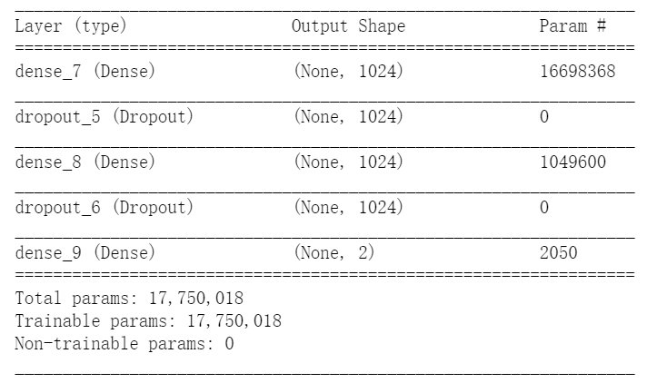
In fact, we didn’t see the implementation of batch normalization, weight decay in their code. The accuracy is soon reach to 94.5% and can hardly get higher. Using 1024 neuron in this trivial task is unnecessary and it converges very fast.
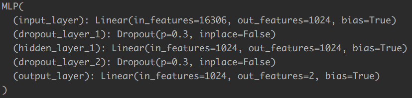
In our PyTorch implementation, we using the same network structure as shown below:
The training process is here:
The Pytorch implementation is here: Identifying Enzymes Using Multi-Layer Neural Network
Gene expression regression
Gene expression data are one of the most common and useful data types in bioinformatics, which can be used to reflect the cellular changes corresponding to different physical and chemical conditions and genetic perturbations. Previously, the most commonly used method is linear regression.
In this example, we use deep learning method to perform gene expression prediction, showing how to perform regression using deep learning. We use the Gene Expression Omnibus (GEO) dataset, which has already gone through the standard normalization procedure. For the regression problem, we use the mean squared error as the loss function. Besides, we also change the activation function of the last layer from Softmax to TanH for this application.