Persistent-Homology-based Machine Learning and its Applications – A Survey
Abstract
A suitable feature representation that can both preserve the data intrinsic information and reduce data complexity and dimensionality is key to the performance of machine learning model. Persistent Homology provides a delicate balance between data simplification and intrinsic structure characterization. However, the combination of PH and machine learning has been hindered greatly by three challenges, namely topological representation of data, PH-based distance measurements or metrics, and PH-based feature representation.
Introduction
Mathematically, feature from geometric analysis can characterize the local structure information very well, but tend to be inundated with details and will result in data complexity. Features generated from traditional topological models, preserve the global intrinsic structure information, but they tend to reduce to much structure information and are rarely used in quantitative characterization.
The essential idea of PH is to employ a filtration procedure, so that each topological generator is equipped with a geometric measurement. In this filtration process, a series of nested simplicial complexes encoded with structural topological information from different scales are produced. It is found that some topological invariants “live” longer in these simplicial complexes, whereas others “die” quickly when filtration value changes. Simply speaking, long-lived Betti numbers usually represent large-sized features. In this way, topological invariants can be quantified by their persistence in the filtration process. The result from PH can be visualized by many methods, including persistent diagram (PD), persistent barcode (PB), persistent landscape, persistent image, etc. When structures are symmetric or have unique topological properties, topological fingerprints can be obtained from the PH analysis and further used in the quantitative characterization of their structures and functions. However, when the systems get more complicated, it becomes more challenging to directly build models on the PB or PD. Instead, machine learning models can be employed to extract the important information or to learn from these topological features.
In algebraic topology, the Betti numbers are used to distinguish topological spaces based on the connectivity of n-dimensional simplicial complexes. For the most reasonable finite-dimensional spaces (such as compact manifolds, finite simplicial complexes or CW complexes), the sequence of Betti numbers is 0 from some point onward (Betti numbers vanish above the dimension of a space), and they are all finite.
With the proper topological simplification, specially-designed PH models can not only preserve the critical chemical and bilogical information, but also enables an efficient topological description of biomolecular interactions.
The unique format of PH outcomes poses a great challenge for a meaningful metrics. To solve this problem, distance measurements or metrics has been considered. These metric definitions are usually based on PD, which can be considered as a two dimensional point distribution. A PD point closed to diagonal line, meaning its death time is only slihtly larger than its birth time, is usually regarded as less “useful” than the ones that are far away from the diagonal line. Given these considerations, pseudo points are introduced and placed on the diagonal lines to guarantee the same number of poins in two PDs for comparison. Further, the Wasserstein distance is used to measure the best possible matching from one PD to the other. And all these distance measurements and metrics can be used in kernel constructions, and further used in machine learning models.
Various PH-based kernels have been proposed. Constructed from PDs and PBs, these kernels can be directly incorporated into kernel-based machine learning methods. PH-based kernels are one way to combine topological information with machine learning models, anoter important way is to generate unique vectors made of topological features and use them in machine learning models.
Topologicl features can be extracted from PDs/PBs. The simplest way of PD/PB-based feature generation is to collect their statistical properties, such as the sum, mean, variance, maximum, minimum, etc. Special opologiccal properties, such as the total Betti number in a certain filtration value, can also be considered as features. A more systematical way of constructing topological feature vectors from PDs/PBs is the binning approach. The essential idea is to discrete the PB or PB into various elements which are then concatenated into a feature vector. Mathematically, binning is just to mploy a Cartesian grid discretization, which is simplest way to discretize a computational domain.
General Pipeline for Persistent-Homology-based Machine Learning
The essential idea for PHML is to extract topological features from the data using PH, and then combine these features with machine learning methods, including both supervised learning and unsupervised learning approaches.
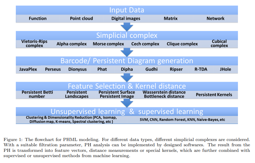
The first step is to construct simplicial complex from the studied data. In topological modeling, we may have various types of data, including functional data, point cloud data, matrixes, networks, images, etc. These data need to be represented by suitable simplicial complexes. Roughly speaking, the simplicial complex can be viewed as a set of combinatorial elements generated from the discretization of spaces.
The second step is the PH analysis. In PH, algebraic tools are used to characterize topological invariants. Unlike traditional topological models, which capture only te intrinsic structure information and tend to ignore all geometric details, PH works as a multiscale topological representation and enables to embed geometric information back into topological invariants. This is achieved through a new idea called filtration. With a suitable filtration process, the persistence of topological invariants can be calculated. The persistece tells you the geometric size of the invariant.
The third step is to extrac meaningful topological features from PH results. We need to transform the PH results into representations, which can be easily incorporated into machine learning models. Two basic approaches are available:
- To generate special PH-based kernels or similarity measurements. These kernels and similarity matrixes can then be combined with PCA, SVM, K-means, spectral clustering, isomap, diffusion map, and etc.
- To generate topological feature vectors from PHA results. Bining approach is the most commonly used approach to discretize the PB or PD into a feature vector.
The last step is to combine the topological features with machine learning algorithms.
Persistent Homology for Dta Modeling and Analysis
Simplicial Complexes
A simplicial complex is a combination of simplexes (单纯形) under certain rules. It can be viewed s a generalization of network or graph model.
Abstract Simplicial Complex
A simplex is the building block for simplicial complex. It can be viewed as a generalization of a triangle or tetrahedron to their higher dimensional counterparts.
Definition 1: A geometric k-simplex \(\sigma^k={v_0, v_1, v_2, \dots, v_k}\) is the convex hull formed by \(k+1\) affinely independent points \(v_0, v_1, v_2, \dots, v_k\) in Euclidean space \(R^d\) as follows,
\[\sigma^k = \left{\lambda_0v_0 + \lambda_1v_1+\dots+\lambda_kv_k | \sum_{i=0}^k \lambda_i=1;0\leq \lambda_i \leq 1, i=0,1,\dots, k \right}\]A face \(\tau\) of k-simplex \(\sigma^k\) is the convex hull of a non-empty subset. We denote it as \(\tau \leq \sigma^k\).
Geometrically, a 0-simplex is a vertex,a 1-simplex is an edge, 2-simplex is a triangle, and a 3-simplex represents a tetrahedron.
Definition 2: A geometric simplicial complex K is a finite set of geometric simplices that satisfy two essential conditions:
- Any face of a simplex from K is also in K
- The intersection of any two simplices in K is either empty or shares faces.
The dimension of K is the maximal dimension of its simplexes. A geometric simplicial complex K is combinatorial set, not a topological space. However, all the points of \(R^d\) that lie in the simplex of K aggregate together to topologize it into a subspace of \(R^d\), known as polyhedron of K.
Graphs and networks, which are comprised of only vertices and edges, can be viewed as a simplicial complex with only 0-simplex and 1-simplex.
Definition 3: An abstrat simplicial complex K is a finite set of elements \(\sigma^k={v_0, v_1, v_2, \dots, v_k}\) called abstract vertices, together with a collection of subsets \((v_{i0}, v_{i1}, v_{i2}, \dots, v_{ik})\) called abstract simplexes, with the property that any subset of a simplex is still a simplex.
For an abstract simplicial complex K, there exists a geometric simplicial complex K’ whose vertices are in one-to-one correspondence with the vertices of K and a subset of vertices being a simplex of K’ is called the geometric realization of K.
Cech Complex and Vietoris-Rips Complex
Let X be a point set in Eucledian space \(R^d\) and \(\mathcal{U}\) is a good cover of X, i.e., \(X \subseteq \cup_{i\in I} \mathcal{U}_i\).
Definition 4: The nerve \(\mathcal{N}\) of \(\mathcal{U}\) is defined by the following two conditions:
- \(\emptyset \in \mathcal{N}\)
- If \(\cap_{j\in J} U_j \neq \emptyset\) for \(J \subseteq I\), then \(J \in \mathcal{N}\)
Theorem 1: (Nerve theorem) The geometric realization of the nerve of \(\mathcal{U}\) is homotopy equivalent to the union of sets in \(\mathcal{U}\).
We can define \(B(X, \epsilon)\) o be the closed balls of radius \(\epsilon\) centered at \(x \in X\), then the union of these balls is a cover of space X and Cech complex is the nerve of this cover.
| Definition 5: The Cech complex with parameter \(\epsilon\) of X is the nerve of the collection of balls \(B(X, \epsilon)\). The Cech complex \(C_\epsilon(X)\) can be represented as \(C_\epsilon(X):={\sigma \in X | \cap_{x\in\sigma} B(X,\epsilon) \neq \emptyset}\). |
Definition 6: The Vietoris-Rips complex (Rips complex) with parameter \(\epsilon\) denoted by \(R_\epsilon (X)\), is the set of all \(\sigma \subseteq X\), such that the largest Euclidean distance between any of its points is at most \(2\epsilon\).
It should be noticed that both Cech complex and Vietoris-Rips complex are abstract simplicial complexes, that are defined on point cloud data in a metric space. However, only Cech complex preserves the homotopy information of the topological spaces formed by the \(\epsilon\) -balls.