Introduction
Motivations
Convolutional Neural Networks
Firstly, GNNs are motivated by convolutional neural networks. We find the keys of CNNs:
- local connection
- shared weights
- use of multi-layer
These are also of great importance in solving problems of graph domain, because
- graphs are the most typical locally connected structure
- shared weights reduce the computational cost compared with traditional spectral graph theory
- multi-layer structure is the key to deal with hierarchical patterns, which captures the features of various sizes
It is straightforward to think of finding the generalization of CNNs to graphs.
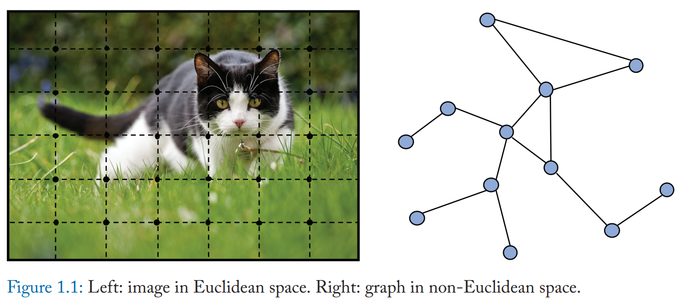
In Figure 1.1, it is hard to define localized convolutional filters and pooling operators, which hinders the transformation of CNN from Euclidean to non-Euclidean domain.
Network Embedding
The graph embedding, which learns to represent graph nodes, edges, or subgraphs in low-dimensional vectors.
Following the idea of representation learning and the success of word embedding, Deep Walk, which is regarded as the first graph embedding method based on representation learning, applies SkipGram model on the generated random walks.
Similar approaches such as node2vec, LINE, and TADW also achieved breakthroughs.
However, these methods suffer from two severe drawbacks:
- no parameters are shared between nodes in the encoder, which leads to computational inefficiency
- the direct embedding methods lack the ability of generalization, which means they cannot deal with dynamic graphs or be generalized to new graphs
Basics of Math and Graph
Linear Algebra
Vectors
The norm of a vector measures its length. The \(L_p\) is defined as follows:
\[||x||_p = (\sum_{i=1}^n|x_i|^p)^{\frac{1}{p}}\]The \(L_1\) norm can be simplified as
\[||x||_1 = \sum_{i=1}^n |x_i|\]In Euclidean space, the \(L_2\) norm is used to measure the length of vectors, where
\[||x||_2 = \sqrt{\sum_{i=1}^n x_i^2}\]The \(L_{infty}\) norm is also called the max norm, as
\[||x||_{\infty} = \max_i |x_i|\]A set of vectors \(x_1, x_2, \dots, x_m\) are linearly independent if and only if there does not exist a set of scalars \(\lambda_1, \lambda_2, \dots, \lambda_m\), which are not all 0, such that
\[\lambda_1 x_1 + \lambda_2 x_2 + \dots \lambda_m x_m = 0\]Matrix
For each \(n \times n\) square matrix \(A\), its determinant is defined as
\[det(A) = \sum_{k_1k_2\dots k_n}(-1)^{\tau (k_1 k_2 \dots k_n)}a_{1k_1} a_{2k2} \dots a_{nkn}\]where \(k_1k_2\dots k_n\) is a permutation of \(1, 2, \dots, n\) and \(\tau(k_1k_2\dots k_n)\) is the inversion number of the permutation \(k_1k_2\dots k_n\), which is the number of inverted sequence in the permutation.
There is a frequently used product between matrices called Hadamard product. The Hadamard product of two matrices \(A, B\) is a matrix \(C), where
\[C_{ij} = A_{ij}B_{ij}\]Tensor
An array with arbitrary dimension. Most matrix operations can also be applied to tensors.
Eigen Decomposition
Let \(A\) be a matrix. A nonzero vector \(v) is called an eigenvector of \(A\) if there exists such scalar \(\lambda\) that
\[Av = \lambda v\]Here scalar \(\lambda\) is an eigenvalue of \(A\) corresponding to the eigenvector \(v\). If matrix \(A\) has n eigenvectors \(v_1, v_2, \dots, v_n\) that are linearly independent, corresponding to the eigenvalue \(\lambda_1, \lambda_2, \dots, \lambda_n\), then it can be deduced that
\[A\begin{bmatrix} v_{1} & v_{2} & \dotsc & v_{n} \end{bmatrix} =\begin{bmatrix} v_{1} & v_{2} & \dotsc & v_{n} \end{bmatrix}\begin{bmatrix} \lambda _{1} & & & \\ & \lambda _{2} & & \\ & & \dotsc & \\ & & & \lambda n \end{bmatrix}\]Let
\[V = \begin{bmatrix}v_{1} & v_{2} & \dots & v_{n}\end bmatrix}\]then it is clear that \(V\) is an invertible matrix. We have the eigen decomposition of \(A\) (also called diagonalization)
\[A = V diag{\lambda} V^{-1}\]It can also be written in the following form:
\[A = \sum_{i=1}^n \lambda_i v_i v_i^\top\]However, not all square matrices can be diagonalized in such form because a matrix may not have as many as \(n\) linear independent eigenvectors. It can be proved that every real symmetric matrix has an eigendecomposition.
The matrix \(A\) and its transpose \(A^\top\) share the same eigen values.
Singular Value Decomposition
As eigendecomposition can only be applied to certain matrices, we introduce the singular value decomposotion, which is a generalization to all matrices.
Singular Value: Let \(r\) denote the rank of \(A^\top A\), then there exist \(r\) positive scalars \(\sigma_1 \geq \sigma_2 \geq \dots \geq \sigma_r \geq 0\) such that for \(1 \leq i \leq r\), \(v_i\) is an eigenvector of \(A^\top A\) with corresponding eigenvalue \(\sigma_i^2\). The r positive scalars \(\sigma_1, \sigma_2, \dots, \sigma_r\) are called singular values of A. Then we have the singular value decomposition:
\[A = U\Sigma V^\top\]where \(U\) and \(V\) are orthogonal matrices and \(\Sigma\) is an \(m \times n\) matrix defined as follows:
\(\Sigma _{ij} =\begin{cases} \sigma _{i} & if\ i\ =\ j\ \leq \ r\\ 0 & otherwise \end{cases}\) f \(AA^\top\), and the eigenvectors of \(A^\top A\) are made up of the column vectors of \(V\).
Probability Theory
Basic Concepts and Formulas
In probability theory, a random variable is a variable that has a random value. If we denote a random value by \(X\), which has two possible values \(x_1\) and \(x_2\), then the probability of \(X\) equals to \(x_1\) is \(P(X=x_1)\). The following equation remains true:
\[P(X=x_1) + P(X=x_2) = 1\]Suppose there is another random variable \(Y\) that has \(y_1\) as a possible value. The probability that \(X=x_1\) and \(Y=y_1\) is written as \(P(X=x_1, Y=y_1)\), which is called the joint probability of \(X=x_1\) and \(Y=y_1\).
The probability of \(X=x_1\) on the condition that \(Y=y_1\), which can be written as \(P(X=x_1 \mid Y=y_1)\). We call this the conditional probability of \(X=x_1\) given \(Y=y_1\). With the concepts above, we can write the following two fundamental rules of probability theory:
\[P(X=x)=\sum_y P(X=x, Y=y)\\ P(X=x, Y=y) = P(Y=y|X=x)P(X=x)\]The former is the sum rule while the latter is the product rule. The modified product rule can be written as:
\[P(Y=y|X=x) = \frac{P(X=x, Y=y)}{P(X=x)} = \frac{P(X=x|Y=y)P(Y=y)}{P(X=x)}\]which is the famous Bayes formula. It also holds for more than two variables:
\[P(X_i = x_i|Y_i = y_i) = \frac{P(Y=y|X_i=x_i)P(X_i=x_i)}{\sum_{j=1}^{n}P(Y=y|X_j=x_j)P(X_j=x_j)}\]Using product rule, we can deduce the chain rule:
\[P(X_1 = x_1, \dots, X_n=x_n)=P(X_1=x_1)\prod_{i=2}^{n}P(X_i=x_i|X_1=x_1, \dots, X_{i-1}=x_{i-1})\]where \(X_1, \dots, X_n\) are n random variables.
The average value of some function \(f(x)\) under a probability distribution \(P(x)\) is called the expectation of \(f(x)\). It can be written as:
\[\mathbb{E}[f(x)] = \sum_x P(x)f(x)\]Usually, \(\mathbb{E}[x]\) stands for the expectation of \(x\).
To measure the dispersion level of \(f(x)\) around its mean value \(\mathbb{E}[f(x)]\), we introduce the variance of \(f(x)\):
\[Var(f(x)) = \mathbb{E}[(f(x) - \mathbb{E}[f(x)])^2] = \mathbb{E}[f(x)]^2 - \mathbb{E}[f(x)]^2\]Covariance expresses the degree to which two variables vary together:
\[Cov(f(x), g(y)) = \mathbb{E}[(f(x) - \mathbb{E}[f(x)])](g(y) - \mathbb{E}[g(y)])\]Probability Distribution
Probability distributions describe the probability of a random variable or several random variables on every state.
Gaussian Distribution: it is also known as normal distribution:
\[N(x|\mu, \sigma^2) = \frac{1}{2\pi \sigma^2} \exp (-\frac{1}{2\sigma^2}(x-\mu)^2)\]where \(\mu\) is the mean of variable \(x\) and \(\sigma^2\) is the variance.
Bernoulli distribution: random variable \(X\) can either be 0 or 1, with a probability \(P(X=1)=p\). Then the distribution function is:
\[P(X=x) = p^x(1-p)^{1-x}, x \in \{0, 1\}\]It is quite obvious that \(\mathbb{E}(X)=p\) and \(Var(X) = p(1-p)\).
Binomial distribution: repeat the Bernoulli experiment for N times and the times that \(X\) equals to 1 is denoted by \(Y\), then
\[P(Y=k) = \begin{pmatrix} N\\ k \end{pmatrix} p^{k}( 1-p)^{N-k}\]is the Binomial distribution satisfying that \(\mathbb{E}(Y)=np\) and \(Var(Y) = np(1-p)\).
Laplace distribution: is described as
\[P(x|\mu, b) = \frac{1}{2b} \exp (-\frac{|x-\mu|}{b})\]Graph Theory
Basic Concepts
A graph is often denoted by \(G=(V, E)\), where \(V\) is the set of vertices and \(E\) is the set of edges. An edge \(e=u, v\) has two endpoints \(u\) and \(v\), which are said to be joined by \(e\). In this case, \(u\) is called a neighbor of \(v\), these two vertices are adjacent. A graph is called a directed graph if all edges are directed. The degree of vertices \(v\), denoted by \(d(v)\), is the number of edges connected with \(v\).
Algebra Representations of Graphs
Adjacency matrix: for a simple graph \(G=(V, E)\) with n-vertices, it can be described by an adjacency matrix \(A \in R^{n\times n}\), where
\[A_{ij} = \begin{cases} 1 & if\ \{v_{i} ,\ v_{j}\} \in E\ and\ i\neq j\\ 0 & otherwise \end{cases}\]It is obvious that such matrix is a symmetric matrix when G is an undirected graph.
Degree matrix: for a graph \(G=(V, E)\) with n-vertices, its degree matrix \(D \in R^{n\times n}\) is a diagonal matrix, where \(D_{ii}=d(v_i)\).
Laplacian matrix: for a simple graph \(G=(V, E)\) with n-vertices, if we consider all edges in G to be undirected, then its Laplacian matrix \(L \in R^{n\times n}\) can be defined as
\[L = D - A\]Thus, we have the elements:
\[L_{ij} =\begin{cases} d( v_{i}) & if\ i\ =\ j\\ -1 & if\ \{v_{i} ,\ v_{j}\} \ \in \ E\ and\ i\ \neq j\\ 0 & otherwise \end{cases}\]Symmetric normalized Laplacian: the symmetric normalized Laplacian is defined as:
\[L^{sym} = D^{-\frac{1}{2}}LD^{-\frac{1}{2}}=I-D^{-\frac{1}{2}}AD^{-\frac{1}{2}}\]The elements are given by:
\[L^{sym}_{ij} =\begin{cases} 1 & if\ i\ =\ j\ and\ d( v_{i}) \neq 0\\ -\frac{1}{\sqrt{d( v_{i}) d( v_{j})}} & if\ \{v_{i} ,\ v_{j}\} \in E\ and\ i\neq j\\ 0 & otherwise \end{cases}\]Random walk normalized Laplacian: it is defined as:
\(L^{rw} = D^{-1}L=I-D^{-1}A\) The elements can be computed by:
\[L^{rw}_{ij} =\begin{cases} 1 & if\ i\ =\ j\ and\ d( v_{i}) \neq 0\\ -\frac{1}{d( v_{i})} & if\ \{v_{i} ,\ v_{j}\} \in E\ and\ i\neq j\\ 0 & otherwise \end{cases}\]Incidence matrix: For a directed graph \(G=(V, E)\) with n-vertices and m-edges, the corresponding incidence matrix is \(M\in R^{n\times n}\), where
\[M_{ij} =\begin{cases} 1 & if\ \exists k\ s.t.\ e_{j} =\{v_{i} ,\ v_{k}\}\\ -1 & if\ \exists k\ s.t.\ e_{j} =\{v_{k} ,\ v_{j}\}\\ 0 & otherwise \end{cases}\]For a undirected graph, the corresponding incidence matrix satisfies that:
\[M_{ij} =\begin{cases} 1 & if\ \exists k\ s.t.\ e_{j} =\{v_{i} ,\ v_{k}\}\\ 0 & otherwise \end{cases}\]Basics of Neural Network
A neural network learns in the following way: initiated with random weights or values, the connections between neurons updates its weights or values by the back propagation algorithm repeatedly till the model performs rather precisely. In the end, the knowledge that a neural network learned is stored in the connections in a digital manner.
Neuron
The basic units of neural networks are neurons, which can receive a series of inputs and return the corresponding output. Where the neuron receives \(n\) inputs \(x_1, \dots, x_n\) with corresponding weights \(w_1, \dots, w_n\) and an offset \(b\).
Several activation functions are shown as follows:
- Sigmoid: \(\sigma(x) = \frac{1}{1 + e^{-x}}\)
- Tanh: \(tanh(x) = \frac{e^x-e^{-x}}{e^x+e^{-x}}\)
- ReLU:
During the training of a neural network, the choice of activation function is usually essential to the outcome.
Back Propagation
During the training of a neural network, the back propagation algorithm is most commonly used. It is an algorithm based on gradient descend to optimize the parameters in a model.
In summary, the process of he back propagation consists of the following two steps:
- Forward calculation: given a set of parameters and an input, the neural network computes the values at each neuron in a forward order.
- Backward propagation: compute the error at each variable to be optimized, and update the parameters with their corresponding partial derivatives in a backward order.
Neural Networks
Feedforward neural network
The FNN usually contains an input layer, several hidden layers, and an output layer. The feedforward neural network has a clear hierarchical structure, which always consists of multiple layers of neurons, and each layer is only connected to its neighbor layers. There are no loops in this network.
Convolutional neural network
FNNs are usually fully connected networks while CNNs preserve the local connectivity. The CNN architecture usually contains convolutional layers, pooling layers, and several fully connected layers. CNNs are widely used in the area of computer vision and proven to be effective in man other research fields.
Recurrent neural network
The neurons in RNNs receive not only signals and inputs from other neurons, but also its own historical information. The memory mechanism in RNN help the model to process series daa effectively. However, the RNN usually suffers from te problem of long-term dependencies. The RNN is widely used in the area of speech and natural language processing.
Graph neural network
The GNN is designed specifically to handle graph-structured data, such as social networks, molecular structures, knowledge graphs.