Introduction to GNN Note 2

Vanilla Graph Neural Networks

We list the limitations of the vanilla GNN in representation capability and training efficiency.

Introduction

The concept of GNN aims to extend existing neural networks for processing graph-structured data.

A node is naturally defined by its features and related nodes in the graph. The target of GNN is to learn a state embedding \(h_v\), which encodes the information of the neighborhood, for each node. The state embedding \(h_v\) is used to produce an output \(o_v\), such as the distribution of the predicted node label.

The vanilla GNN model deals with the undirected homogeneous graph where each node in the graph has its input features \(x_v\) and each edge may also have its features.

Model

Given the input features of nodes and edges, next we will talk about how the model obtains the node embedding \(h_v\) and the output embedding \(o_v\).

In order to update the node state according to the input neighborhood, there is a parametric function \(f\), called local transition function, shared among all nodes. In order to produce the output of the node, there is a parametric function \(g\), called local output function. Then, \(h_v\) and \(o_v\) are defined as follows:

where \(x\) denotes the input feature and \(h\) denotes the hidden state. \(co[v]\) is the set of edges connected to node \(v\) and \(ne[v]\) is set of neighbors of node \(v\). So that \(x_v, x_{co[v]}, h_{ne[v]}, x_{ne[v]}\) are the features of \(v\), the features of its edges, the states and the features of the nodes in the neighborhood of \(v\), respectively.

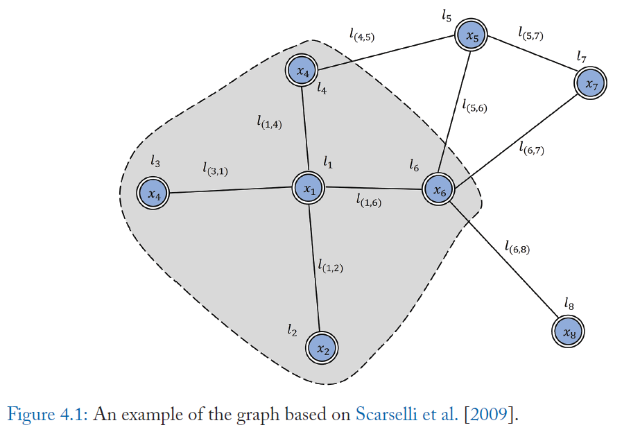
In the example of node \(l_1\), \(x_{l_1}\) is the input feature of \(l_1\). \(co[l_1]\) contains edges \(l_{(1, 4)}, l_{(1, 6)}, l_{(1, 2)}, l_{(3, 1)}\). \(ne[l_1]\) contains nodes \(l_2, l_3, l_4, l_6\).

Let H, O, X, and \(X_N\) be the matrices constructed by stacking all the states, all the outputs, all the features, and all the node features, respectively. Then we have a compact form as:

where F, the global transition function, and G is the global output function. The value of H is the fixed point and is uniquely defined with the assumption that F is a contraction map.

GNN uses the classic iterative scheme to compute the state:

where \(H^t\) denotes the tth iteration of H. The dynamical system converges exponentially fast to the solution for any initial value of \(H(0)\).

The next question is how to learn the parameters of the local transition function \(f\) and local output function \(g\). With the target information (\(t_v\) for a specific node) for the supervision, the loss can be written as:

where p is the number of supervised nodes. The learning algorithm is based on a gradient descent strategy and is composed of the following steps:

• The states \(h^t_v\) are iteratively updated by \(h_v = f(x_v, x_{co[v]}, h_{ne[v]}, x_{ne[v]}) \) until a time step \(T\). Then we obtain an approximate fixed point solution of \(H = F(H, X)\): \(H(T) \approx H\)
• The gradient of weights \(W\) is computed from the loss
• The weights \(W\) are updated according to the gradient computed in the last step.

After running the algorithm, we can get a model trained for a specific supervised/semi-supervised task as well as hidden states of nodes in the graph. The vanilla GNN model provides an effective way to model graphic data and it is the first step toward incorporating neural networks into graph domain.

Limitations

• It is computationally inefficient to update the hidden states of nodes iteratively to get the fixed point. The model needs \(T\) steps of computation to approximate the fixed point. If relaxing the assumption of the fixed point, we can design a multi-layer GNN to get a stable representation of the node and its neighborhood.
• Vanilla GNN uses the same parameters in the iteration while most popular neural networks use different parameters in different layers.
• There are also some informative features on the edges which cannot be effectively modeled in the vanilla GNN. How to learn the hidden sates of edges is also an important problem.
• If \(T\) is pretty large, it is unsuitable to use the fixed points if we focus on the representation of nodes instead of graphs because the distribution of representation in the fixed point will be much more smooth in value and less informative.

Graph Convolutional Network

GCNs aim to generalize convolutions to the graph domain. As CNNs have achieved great success in the area of deep learning, it is intuitive to define the convolution operation on graphs. Advances in this direction are often categorized as spectral approaches and spatial approaches.

Spectral Methods

Spectral approaches work with a spectral representation of the graphs.

Spectral Network

The convolution operation is defined in the Fourier domain by computing the eigendecomposition of the graph Laplacian. The operation can be defined as the multiplication of signal \(x \in R\) with a filter \(g_\theta = diag(\theta)\) parameterized by \(\theta\):

where \(U\) is the matrix of eigenvectors of the normalized graph Laplacian \(L=I_N - D^{-\frac{1}{2}}AD^{-\frac{1}{2}} = U\Lambda U^\top\). \(D\) is the degree matrix and \(A\) is the adjacency matrix of the graph, with a diagonal matrix of its eigenvalues \(\Lambda\).

This operation results in potentially intense computations and non-spatially localized filters.

ChebNet

Hammond suggest that \(g_\theta(\Lambda)\) can be approximated by a truncated expansion in terms of Chebyshev polynomials \(T_k(x)\) up to \(K^{th}\) order. Thus, the operation is:

with \(\tilde{L} = \frac{2}{\lambda max}L - I_N \cdot\). \(\lambda_{max}\) denotes the largest eigenvalue of \(L\). \(\theta \in R\) is now a vector of Chebyshev coefficients. The Chebyshev polynomials are defined as \(T_k(x) = 2xT_{k-1}(x) - T_{k-2}(x)\) with \(T_0(x)=1, T_1(x)=x\). It can be observed that the operation is K-localized since its a Kth-order polynomial in the Laplacian.

ChebNet uses this K-localized convolution to define a convolutional neural network which could remove the need to compute the eigenvectors of the Laplacian.

GCN

Kipf limit the layer-wise convolution operation to \(K=1\) to alleviate the problem of overfitting on local neighborhood structures for graphs with very wide node degree distributions. It further approximates \(\lambda_{max} \approx 2\) and the equation simplifies to:

with two free parameters \(\theta_0’\) and \(\theta_1’\). After constraining the number of parameters with \(\theta = \theta_0’=-\theta_1’\), we can obtain the following expression:

Note that stacking this operator could lead to numerical instabilities and exploding/vanishing gradients. Kipf introduced the renormalization trick: \(I_N + D^{-\frac{1}{2}}AD^{-\frac{1}{2}} \rightarrow \tilde{D}^{-\frac{1}{2}}\tilde{A}\tilde{D}^{-\frac{1}{2}} \) with \(\tilde{A} = A+I_N\) and \(\tilde{D}{ii} = \sum_j \tilde{A}{ij}\). Finally, they generalize the definition to a signal \(X \in R^{N \times C}\) with C input channels and F filters for feature maps as follows:

where \(\Theta \in R^{C\times F}\) is a matrix of filter parameters and \(Z \in R^{N\times F}\) is the convolved signal matrix.

As a simplification of spectral methods, the GCN model could also be regarded as a spatial method.

AGCN

There may have implicit relations between different nodes and the Adaptive Graph Convolution Network is proposed to learn the underlying relations. AGCN learns a “residual” graph Laplacian \(L_{res}\) and add it to the original Laplacian matrix:

where \(\alpha\) is a parameter. \(L_{res}\) is computed by a learned graph adjacency matrix \(\hat{A}\):

and \(\hat{A}\) is computed via a learned metric. The idea behind the adaptive metric is that Euclidean distance is not suitable for graph structured data and the metric should be adaptive to the task and input features. AGCN uses the generalized Mahalanobis distance:

where M is a learned parameter that satisfies \(M=W_dW_d^T\) is the transform basis to the adaptive space. Then AGCN calculates the Gaussian kernel and normalize G to obtain the dense adjacency matrix \(\hat{A}\):

Spatial Methods

In all of the spectral approaches mentioned above, the learned filters depend on the Laplacian eigenbasis, which depends on the graph structure. That means a model trained on a specific structure could not be directly applied to a graph with a different structure.

In contrast, spatial approaches define convolutions directly on the graph, operating on spatially close neighbors.

The major challenge of spatial approaches is defining the convolution operation with differently sized neighborhoods and maintaining the local invariance of CNNs.

Neural FPS

Duvenaud use different weight matrices for nodes with different degrees:

where \(W_t^{ \mid N_v\mid}\) is the weight matrix for nodes with degree \( \mid N_v \mid \) at layer t, \(N_v\) denotes the set of neighbors of node v, \(h_v^t\) is the embedding of node v at layer t.

The model first adds the embeddings from itself as well as its neighbors, then it uses \(W_t^{ \mid N_v \mid}\) to do the transformation. The model defines different matrices \(W_t^{\mid N_v \mid}\) for nodes with different degrees.

The main drawback of the method is that it cannot be applied to large-scale graphs with more node degrees.

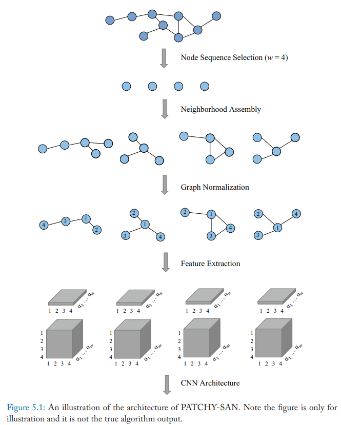
Patchy-SAN

The model first selects and normalizes exactly k neighbors for each node. Then the normalized neighborhood serves as the receptive field and the convolutional operation is applied.

The method has four steps:

• Node Sequence Selection: This method selects a sequence of nodes for processing. It first uses a graph labeling procedure to get the order of the nodes and obtain the sequence of the nodes. Then the method uses a stride s to select nodes from the sequence until a number of w nodes are selected.
• Neighborhood Assembly: The receptive fields of nodes selected from last step are constructed. The neighbors of each node are the candidates and the model ses a simple BFS search to collect k neighbors for each node. It first extracts the 1-hop neighbors of the node, then it considers high-order neighbors until the total number of k neighbors are extracted.
• Graph Normalization: The algorithm aims to give an order to nodes in the receptive field, so that this step maps from the unordered graph space to a vector space. This is the most important step and the idea behind this step is to assign nodes from two different graphs similar relative positions if they have similar structural roles.
• Convolutional Architecture: After the receptive fields are normalized in last step, CNN architectures can be used. The normalized neighborhoods serve as receptive fields and node and edge attributes are regarded as channels.

DCNN

Diffusion-convolutional neural networks (DCNNs). Transition matrices are used to define the neighborhood for nodes in DCNN. For node classification, it has

where \(X\) is an \(N\times F\) tensor of input features (N number of nodes and F is the number of features). \(P*\) is an \(N\times K\times N\) tensor which contains the power series \({P, P^2, \dots, P^k}\) of matrix \(P\). And \(P\) is the degree-normalized transition matrix from the graphs adjacency matrix \(A\). Each entity is transformed to a diffusion convolutional representation which is a \(K\times F\) matrix defined by \(K\) hops of graph diffusion over \(F\) features. And then it will be defined by a \(K\times F\) weight matrix and a nonlinear activation function \(\sigma\). Finally, \(H\) (which is \(N\times K\times F\)) denotes the diffusion representations of each node in the graph.

As for graph classification, DCNN simply takes the average of nodes’ representation,

and \(1_N\) here is an \(N\times 1\) vector of ones. DCNN can also be applied to edge classification tasks, which requries converting edges to nodes and augmenting the adjacency matrix.

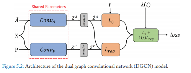
DGCN

The dual graph convolutional network (DGCN) is jointly considered the local consistency and global consistency on graphs. It uses two convolutional networks to capture the local/global consistency and adopts an unsupervised loss to ensemble them. The first convolutional network is the same as GCN. And the second network replaces the adjacency matrix with positive point-wise mutual information (PPMI) matrix:

where \(X_p\) is the PPMI matrix and \(D_p\) is the diagonal degree matrix of \(X_p\), \(\sigma\) is a nonlinear activation function.

The motivations of jointly using the two perspectives are:

1. GCN models the local consistency, which indicates that nearby nodes may have similar labels, and
2. PPMI module models the global consistency which assumes that nodes with similar context may have similar labels.

The local consistency convolution and global consistency convolution are named as \(Conv_A\) and \(Conv_P\).

They further ensemble these two convolutions via the final loss function. It can be written as:

\(\lambda(t)\) is the dynamic weight to balance the importance of these two loss functions. \(L_0(Conv_A)\) is he supervised loss function with given node labels. If we have \(c\) different labels to predict, \(Z^A\) denotes the output matrix of \(Conv_A\) and \(\hat{Z}^A\) denotes the output of \(Z^A\) after a softmax operation, then the loss \(L_0(Conv_A)\), which is the cross-entropy error, can be written as:

where \(y_L\) is the set of training data indices and Y is the ground truth.

The calculation of \(L_{reg}\) can be written as:

where \(\hat{Z}^P\) denotes the output of \(Conv_P\) after the softmax operation. Thus, \(L_{reg}(Conv_A, Conv_P)\) is the unsupervised loss function to measure the differences between \(\hat{Z}^P\) and \(\hat{Z}^A\).

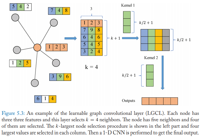
LGCN

Gao propose the learnable graph convolutional networks (LGCN). The network is based on the learnable graph convolutional layer (LGCN) and the sub-graph training strategy.

LGCN leverages CNNs as aggregators. It performs max pooling on nodes’ neighborhood matrices to get top-k feature elements and then applies 1-D CNN to compute hidden representations. The propagation step of LGCL is formulated as:

where \(A\) is the adjacency matrix, \(g(\cdot)\) is the k-largest selection operation, and \(c(\cdot)\) denotes the regular 1-D CNN.

The model uses the k-largest node selection operation to gather information for each node. For a given node \(x\), the features of its neighbors are firstly gathered; suppose it has n neighbors and each node has \(c\) features, then a matrix \(M \in R^{n\times c}\) is obtained. If n is less than k, then M is padded with columns of zeros. Then the k-largest node selection is conducted that we rank the values in each column and select the top-k values. After that, the embedding of the node x is inserted into the first row of the matrix and finally we get a matrix \(\hat{M} \in R^{(k+1)\times c}\).

After the matrix \(\hat{M}\) is obtained, then the model uses the regular 1D CNN to aggregate the features. The function \(c(\cdot)\) should take a matrix of \(N\times (k+1)\times C\) as input and output a matrix of dimension \(N\times D\) or \(N\times 1\times D\).

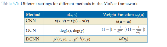
MoNet

Monti proposed a spatial-domain model (MoNet) on non-Euclidean domains which could generalize several previous techniques. The Geodesic GNN (GCNN) and Anisotropic CNN (ACNN) on manifolds or GCN and DCNN on graphs could be formulated as particular instances of MoNet.

We use \(x\) to denote the node in the graph and \(y \in N_x\) to denote the neighbor node of \(x\). The MoNet model computes the pseudo-coordinates \(u(x, y)\) between the node and its neighbor and uses a weighting function among these coordinates:

where the parameters are \(w_\Theta(u)=(w_1(u), \dots, w_J(u))\) and \(J\) represents the size of the extracted patch. Then a spatial generalization of the convolution on non-Euclidean domains is defined as:

The other methods can be regarded as a special case with different coordinates \(u\) and weight function \(w(u)\).

GraphSAGE

Hamilton proposed the GraphSAGE, a general inductive framework. The framework generates embeddings by sampling and aggregating features from a node’s local neighborhood. The propagation step of GraphSAGE is:

where \(W^t\) is the parameter at layer t.

Hamilton suggest three aggregator functions:

• Mean aggregator
• LSTM aggregator
• Pooling aggregator

Graph Attention Networks

The attention mechanism has been successfully used in many sequence-based tasks. Compared with GCN which treats all neighbors of a node equally, the attention mechanism could assign different attention score to each neighbor, thus identifying more important neighbors. It is intuitive to incorporate the attention mechanism into the propagation steps of GNN.

Graph Attention Network (GAT)

GAT incorporates the attention mechanism into the propagation steps. It follows the self-attention strategy and the hidden state of each node is computed by attending over its neighbors.

Graph attention layer is used to construct arbitrary graph attention networks by stacking this layer. The layer computes the coefficients in the attention mechanism of the node pair \((i, j)\) by:

where \(\alpha_{ij}\) is the attention coefficient of node j to i, \(N_i\) represents the neighborhoods of node i in the graph. The input node features are denoted as \(h={h_1, h_2, \dots, h_N}, h_i\in R^F\), where N is the number of nodes and F is the dimension, the output node features are denoted as \(h’ = {h_1’, h_2’, \dots, h_N’}, h_i’ \in R^{F’}\). \(W \in R^{F’\times F}\) is the weight matrix of a shared linear transformation which applied to every node, \(a \in R^{2F’}\) is the weight vector. It is normalized by a softmax function and the LeakyReLU nonlinearity is applied.

Then the final output features of each node can be obtained by (after applying a nonlinearity \(\sigma\)):

Moreover, the layer utilizes the multi-head attention to stabilize the learning process. It applies K independent attention mechanisms to compute the hidden states and then concatenates their features, resulting in the following two output representations:

where \(\alpha ^{k}_{ij}\) is normalized attention coefficient computed by the kth attention mechanism, \(\coprod\) is the concatenation operation.

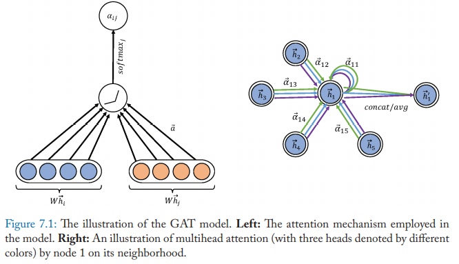
The attention architecture has several properties:

• the computation of the node-neighbor pairs is parallelizable thus the operation is efficient
• it can deal with nodes with different degrees and assign corresponding weights to their neighbors
• it can be applied to the inductive learning problems easily

GAT outperforms GCN in several tasks.

GaAN

Gated Attention Network (GaAN) also uses the multi-head attention mechanism. The difference between the attention aggregator in GaAN and the one in GAT is that GaAN uses the key-value attention mechanism and the dot product attention while GAT uses a fully connected layer to compute the attention coefficients.

GaAN assigns different weights for different heads by computing an additional soft gate. This aggregator is called the gated attention aggregator. GaAN uses a convolutional network that takes the features of the center node and it neighbors to generate gate values. As a result, it could outperform GAT as well as other GNN models with different aggregators in the inductive node classification problem.

• Previous
  Introduction to GNN Note 1
• Next
  Introduction to GNN Note 3