Lecture: Markov Decision Process
Learning Goals
- Understand the Agent-Environment interface
- Understand what MDPs (Markov Decision Processes) are and how to interpret transition diagrams
- Understand Value Functions, Action-Value Functions, and Policy Functions
- Understand the Bellman Equations and Bellman Optimality Equations for value functions and action-value functions
Markov Processes
Introduction to MDPs
Markov decision processes formally describe an environment for reinforcement learning, where the environment is fully observable: the current state completely characterises the process.
Almost all RL problems can be formalised as MDPs.
最优控制问题可以描述成连续MDPs; 部分观测环境可以转化成POMDPs; 赌博机问题是只有一个状态的MDPs。
Markov Property
Definition: A state \(s_t\) is Markov if and only if
\[\mathbb{P}[s_{t+1} \mid s_t] = \mathbb{P}[s_{t+1} \mid s_1, \dots, s_t]\]The state captures all relevant information from the history. Once the state is known, the history may be thrown away. The state is sufficient statistic of the future.
这里要求环境全观测。
State Transition Matrix
For a Markov state \(s\) and successor state \(s’\), the state transition probability is defined by:
\[\mathcal{P}_{ss'} = \mathbb{P}[s_{t+1} = s' \mid s_t = s]\]State transition matrix \(\mathcal{P}\) defines transition probabilities from all states \(s\) to all successor state \(s’\).
\[\mathcal{P} = \begin{bmatrix} \mathcal{P}_{11} & \cdots & \mathcal{P}_{1n}\\ \vdots & \ & \vdots \\ \mathcal{P}_{n1} & \cdots & \mathcal{P}_{nn} \end{bmatrix}\]where each row of the matrix sums to 1.
\[\mathcal{P}(s' \mid s) = \mathbb{P}[s_{t+1} = s' \mid s_t = s]\]\(n\)表示状态的个数; \(\mathcal{P}\) 代表了整个状态转移的集合 每行元素相加等于1。 也可以将状态转移概率写成函数的形式:
\[\sum_{s'} \mathcal{P}(s' \mid s) = 1\ or\ \inf_{s'}\mathcal{P}(s' \mid s) = 1\]其中:
Episode
A sequence process from state \(s_1\) to the terminal state \(s_t\) is called an episode.
An episodic task is always ended up with a terminal state.
A continuing task is executing infinitely, without terminal state.
Markov Process
A Markov process is a memoryless random process, i.e. a sequence of random states \(s_1, s_2, \cdots \) with the Markov property.
Definition: A Markov Process (or Markov Chain) is a tuple \(\left< \mathcal{S}, \mathcal{P} \right> \)
- \(\mathcal{S}\) is a finite set of states
- \(\mathcal{P}\) is a state transition probability matrix: \(\mathcal{P}{ss’} = \mathbb{P}[s{t+1} = s’ \mid s_t=s]\)
虽然我们有时候并不知道\(\mathcal{P}\)的具体值,但是通常我们假设 \(\mathcal{P}\) 存在且稳定的。
Markov Chain
Let \(\s_t \in \mathcal{S}\), and if \(\mathcal{S}\) is finite (countable), we call the Markov Process with this countable state space Markov Chain.
Generating Patterns
Deterministic Patterns
A system that every state relies on the previous state. The system is deterministic.
Non-deterministic Patterns
Markov Assumption: The current state is only relies on some previous states.
But it not always accurate.
对于有 \(M\) 个状态的一阶马尔科夫模型,共有 \(M^2\) 个状态转移,因为任何一个状态都有可能是所有状态的下一个转移状态。每一个状态转移都有一个概率值,称为状态转移概率。 由此,\(M^2\) 个概率也可以用一个状态转移矩阵表示。注意这些概率并不随时间变化而不同。
Hidden Markov
Markov Reward Processes
Introduction
A Markov chain with values.
Definition: A Markov Reward Process is a tuple \(\left< \mathcal{S}, \mathcal{P}, \mathcal{R}, \gamma \right> \)
- \(\mathcal{S}\) is a finite set of states
- \(\mathcal{P}\) is a state transition probability matrix: \(\mathcal{P}{ss’} = \mathbb{P}[s{t+1} = s’ \mid s_t=s]\)
- \(\mathcal{R}\) is a reward function, \(\mathcal{R}s=\mathbb{E}[r{t+1} \mid s_t = s] \)
- \(\gamma\) is a discount factor, \(\gamma \in [0, 1]\)
Return
Definition: The return \(G_t\) is the total discounted reward from time-step \(t\)
\[G_t = R_{t+1} + \gamma R_{t+2} + \dots = \sum_{k=0}^{\infty} \gamma^k R_{t+k+1}\]- The discount \(\gamma \in [0, 1]\) is the present value of future rewards
- The value of receiving reward \(R\) after \(k+1\) time-steps is \(\gamma^k R\)
- This value immediate reward above delayed reward
- \(\gamma\) close to 0 leads to myopic evaluation
- \(\gamma\) close to 1 leads to far-sighted evaluation
奖励是针对状态的,回报是针对片段的。
Value Function
The value function \(v(s)\) gives the long-term value of state \(s\).
Definition: The state value function \(v(s)\) of an MRP is the expected return starting from state \(s\)
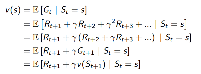
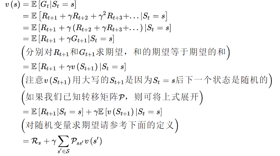
\[v(s) = \mathbb{E}[G_t \mid s_t=s]\]值函数存在的意义:回报值是一次片段(or一次采样)的结果,存在很大的样本偏差; 回报值的角标是 \(t\) ,值函数关注的是状态 \(s\) ,所以又被称为状态价值函数。
Bellman Equation for MRPs
The value function can be decomposed into two parts:
- immediate reward \(R_{t+1}\)
- discounted value of successor state \(\gamma v(S_{t+1})\)
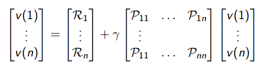
The Bellman equation can be expressed concisely using matrices:
\[v = \mathcal{R} + \gamma \mathcal{P}v\]虽然都是从相同的初始状态开始,但是不同的片段有不同的回报值,而值函数是它们的期望值。
where \(v\) is a column vector with one entry per state
The bellman equation is a linear equation. It can be solved directly:
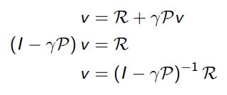
计算复杂度是\(O(n^3)\),\(n\)是状态数量
Direct solution only possible for small MRPs. There are many iterative methods for large MRPs:
- Dynamic Programming
- Monte-Carlo Evaluation
- Temporal-Difference Learning
Markov Decision Process
A Markov decision process (MDP) is a Markov reward process with decisions. It is an environment in which all states are Markov.
MP和MRP中,我们都是作为观察者,去观察其中的状态转移现象,去计算回报值 对于一个RL问题,我们更希望去改变状态转移的流程,去最大化回报值
Definition: A Markov Decision Process is a tuple \(\left< \mathcal{S}, \mathcal{A}, \mathcal{P}, \mathcal{R}, \mathcal{\gamma} \right> \)
- \(\mathcal{S}\) is a finite set of states
- \(\mathcal{A}\) is a finite set of actions
- \(\mathcal{P}\) is a state transition probability matrix: \(\mathcal{P}{ss’}^a = \mathbb{P}[s{t+1} = s’ \mid s_t=s, a_t=a]\)
- \(\mathcal{R}\) is a reward function, \(\mathcal{R}s^a=\mathbb{E}[r{t+1} \mid s_t = s, a_t = a]\)
- \(\gamma\) is a discount factor, \(\gamma \in [0, 1]\)
看起来很类似马尔科夫奖励过程,但这里的 \(\mathcal{P}\) 和 \(\mathcal{R}\) 都与具体的行为 \(a\) 对应,而不像马尔科夫奖励过程那样仅对应于某个状态。
Policies
Definition: A policy \(\pi\) is a distribution over actions given states:
\[\pi(a \mid s) = \mathbb{P}[a_t = a \mid s_t = s]\]A policy fully defines the behavior of an agent. MDP policies depend on the current state. Policies are stationary (time-independent).
\[a_t ~ \pi(\cdot \mid s_t), \forall t>0\]个体可以随着时间更新策略 如果策略的概率分布输出都是 one-hot 的,那么称为确定性策略,否则即为随机策略
Given an MDP \(\mathcal{M}\) and a policy \(\pi\), the state sequence \(s_1, s_2, \cdots \) is a Markov process \(\left< \mathcal{S}, \mathcal{P}^\pi \right>\). The state and reward sequence \(s_1, r_2, s_2, \cdots\) is a Markov reward process \(\left< \mathcal{S}, \mathcal{P}^\pi, \mathcal{R}^\pi, \gamma \right>\), where:
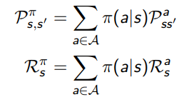
在执行策略 \(\pi\) 时,状态从 \(s\) 转移至 \(s’\) 的概率等于一系列概率的和,这一系列概率指的是在执行当前策略时,执行某一个行为的概率与该行为能使状态从 \(s\) 转移至 \(s’\) 的概率的乘积。
当前状态 \(s\) 下执行某一指定策略得到的即时奖励是该策略下所有可能行为得到的奖励与该行为发生的概率的乘积的和。
Value Function
Definition: The state-value function \(v_\pi (s)\) of an MDP is the expected return starting from state \(s\), and then following policy \(\pi\):
\[v_\pi(s) = \mathbb{E}_\pi [G_t \mid s_t = s]\]在执行当前策略 \(\pi\) 时,衡量个体处在状态 \(s\) 时的价值大小
策略是静态的、关于整体的概念,不随状态改变而改变 变化的是在某一个状态时,依据策略可能产生的具体行为,因为具体的行为是有一定的概率的 策略就是用来描述各个不同状态下执行各个不同行为的概率
Definition: The action-value function \(q_\pi (s, a)\) is the expected return starting from state \(s\), taking action \(a\), and then following policy \(\pi\):
\[q_\pi(s, a) = \mathbb{E}_\pi [G_t \mid s_t = s, a_t = a]\]在遵循当前策略 \(\pi\) 时,衡量对当前状态执行行为 \(a\) 的价值大小
Bellman Expectation Equation
The state-value function can again be decomposed into immediate reward plus discounted value of successor state:
\[v_\pi (s) = \mathbb{E}_\pi [R_{t+1} + \gamma v_\pi (s_{t+1}) \mid s_t = s]\]\[v_\pi (s) = \sum_{a\in \mathcal{A}} \pi(a \mid s) q_\pi (s, a)\]在遵循策略 \(\pi\) 时,状态 \(s\) 的价值体现为在该状态下遵循某一策略而采取所有可能行为的价值按行为发生概率的乘积求和
The action-value function can similarly be decomposed:
\[q_\pi (s, a) = \mathbb{E}_\pi [R_{t+1} + \gamma q_\pi(s_{t+1}, a_{t+1} \mid s_t = s, a_t = a]\]\[q_\pi (s, a) = \mathcal{R}_s^a + \gamma \sum_{s'\in\mathcal{S}} \mathcal{P}_{ss'}^a v_\pi (s')\] \[v_\pi (s) = \sum_{a\in \mathcal{A}} \pi(a \mid s) (\mathcal{R}_s^a + \gamma \sum_{s'\in\mathcal{S}} \mathcal{P}_{ss'}^a v_\pi (s'))\] \[q_\pi (s, a) = \mathcal{R}_s^a + \gamma \sum_{s'\in\mathcal{S}} \mathcal{P}_{ss'}^a \sum_{a'\in \mathcal{A}} \pi(a' \mid s') q_\pi (s', a')\]某一个状态下采取一个行为的价值,可以分为两部分:其一是离开这个状态的价值,其二是所有进入新的态的价值与其转移概率乘积的和。
Matrix Form:
\[v_\pi = \mathcal{R}^\pi + \gamma \mathcal{P}^\pi v_\pi\]Optimal Value Function
Definition: The optimal state-value function \(v_* (s)\) is the maximum value function over all policies:
\[v_* (s) = \max_\pi v_\pi (s)\]The optimal action value function \(q_* (s, a)\) is th maximum action-value function over all policies:
\[q_*(s, a) = \max_\pi q_\pi (s, a)\]The optimal value function specifies the best possible performance in the MDP. An MDP is solved when we know the optimal value function.
Optimal Policy
Define a partial ordering over policies:
\[\pi \geq \pi' if v_\pi(s) \geq v_{\pi'}(s), \forall s\]Theorem: For any MDP:
- There exists an optimal policy \(\pi_\) that is better than or equal to all other policies, \(\pi_ \req \pi, \forall \pi\)
- All optimal policies achieve the optimal value function, \(v_{\pi_}(s) = v_(s)\)
- All optimal policies achieve the optimal action-value function, \(q_\pi_(s, a) = q_(s, a)\)
Finding an Optimal Policy
An optimal policy can be found by maximising over \(q_*(s, a)\):
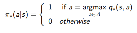
There is always a deterministic optimal policy for any MDP. If we known \(q_*(s,a)\), we immediately have the optimal policy.
Bellman Optimality Equation for \(v_*\)
\[v_*(s) = \max_a q_*(s, a)\] \[v_\pi (s) = \max_a \mathcal{R}_s^a + \gamma \sum_{s'\in\mathcal{S}} \mathcal{P}_{ss'}^a v_* (s')\]假设最优策略是确定性的策略,那么 \(\pi_* (s, a)\) 是one-hot的形式,那么我们只需取最大的 \(q_{\pi_}(s,a)\) 就可以了。又因为所有的最优策略具有相同的行为价值函数,即 \(q_{\pi_}(s, a) = q_*(s,a)\)
Bellman Optimality Equation for \(Q_*\)
\[q_*(s,a) = \mathcal{R}_s^a + \gamma \sum_{s'\in\mathcal{S}} \mathcal{P}_{ss'}^a v_* (s')\] \[q_\pi (s, a) = \mathcal{R}_s^a + \gamma \sum_{s'\in\mathcal{S}} \mathcal{P}_{ss'}^a \max_{a'} q_* (s', a')\]贝尔曼最优方程本质上就是利用了 \(\pi_\) 的特点,将求期望的算子转化成了 \(\max_a\) 在贝尔曼期望方程中, \(\pi\) 是已知的,而在贝尔曼最优方程中, \(\pi_\) 是未知的 解贝尔曼期望方程的过程即对应了评价,解贝尔曼最优方程的过程即对应了优化
Sloving the Bellman Optimality Equation
Bellman Optimality Equation is non-linear. There is no closed form solution in general. But there are many iterative solution methods like Value Iteration, Policy Iteration, Q-learning, Sarsa and so on.
Extensions to MDPs
- Infinite and continuous MDPs
- Partially observable MDPs
- Undiscounted, average reward MDPs
Summary
- Agent & Environment Interface:
- At each step \(t\) the agent receives a state \(s_t\)
- performs an action \(a_t\)
- and receives a reward \(r_{t+1}\)
- The action is chosen according to a policy function \(\pi\)
- The total return \(G_t\) is the sum of all rewards starting from time \(t\)
- Future rewards are discounted at a discount rate \(\gamma^k\)
- Markov property:
- The environment’s response at time \(t+1\) depends only on the state and action representations at time \(t\)
- The future is independent of the past given the present.
- Even if an environment doesn’t fully satisfy the Markov property we still treat it as if it is
- and try to construct the state representation to be approximately Markov.
- Markov Decision Process (MDP):
- Defined by a state set \(S\)
- action set \(A\)
- and one-step dynamics \(p(s’,r \mid s,a)\).
- In practice, we often don’t know the full MDP (but we know that it’s some MDP).
- The Value Function \(v(s)\) estimates how “good” it is for an agent to be in a particular state \(s\)
- More formally, it’s the expected return \(G_t\) given that the agent is in state \(s\)
- \(v(s) = E[G_t \mid S_t = s]\)
- Note that the value function is specific to a given policy \(\pi\).
- Action Value function: \(q(s, a)\) estimates how “good” it is for an agent to be in state \(s\) and take action \(a\).
- Similar to the value function, but also considers the action.
- The Bellman equation expresses the relationship between the value of a state and the values of its successor states
- It can be expressed using a “backup” diagram.
- Bellman equations exist for both the value function and the action value function.
- Value functions define an ordering over policies
- A policy \(p_1\) is better than \(p_2\) if \(v_{p_1}(s) >= v_{p_2}(s)\) for all states \(s\).
- For MDPs, there exist one or more optimal policies that are better than or equal to all other policies.
- The optimal state value function \(v*(s)\) is the value function for the optimal policy.
- Same for \(q*(s, a)\).
- The Bellman Optimality Equation defines how the optimal value of a state is related to the optimal value of successor states.
- It has a “max” instead of an average.