David Silver - Reinforcement Learning Note 3

Lecture: Planning by Dynamic Programming

Learning Goals

• Understand the difference between Policy Evaluation and Policy Improvement and how these processes interact
• Understand the Policy Iteration Algorithm
• Understand the Value Iteration Algorithm
• Understand the Limitations of Dynamic Programming Approach

Introduction

Dynamic: Sequential or temporal component to the problem. Programming: Optimizing a “program”, i.e., a policy

A method for solving complex problems, by breaking them down into subproblems: solve the subproblems and combine solutions to subproblems.

Requirements for Dynamic Programming

Dynamic Programming is a very general solution for problems which have two properties:

• Optimal substructure
  • Principle of optimality applies
  • Optimal solution can be decomposed into subproblems
• Overlapping subproblems
  • Subproblems recur many times
  • Solutions can be cached and reused

Markov decision processes satisfy both properties:

• Bellman equation gives recursive decomposition
• Value function stores and reuses solutions

Planning by Dynamic Programming

Dynamic programming assumes full knowledge of the MDP. It is used for planning in an MDP.

For prediction:

• Input: MDP \(\left< \mathcal{S}, \mathcal{A}, \mathcal{P}, \mathcal{R}, \mathcal{\gamma}, \right>\) and policy \(\pi\)
• or: MRP \(\left< \mathcal{S}, \mathcal{P}^\pi, \mathcal{R}^\pi, \mathcal{\gamma}, \right>\)
• Output: value function \(v_\pi\)

For control:

• Input: MDP \(\left< \mathcal{S}, \mathcal{A}, \mathcal{P}, \mathcal{R}, \mathcal{\gamma}, \right>\)
• Output: optimal value function \(v_\) and optimal policy \(\pi_\)

Policy Evaluation

Iterative Policy Evaluation

Problem: evaluate a given policy \(\pi\) Solution: iterative application of Bellman Expectation backup

也就是解决“预测”问题

Using synchronous backups:

• At each iteration \(k+1\)
• For all states \(s \in \mathcal{S}\)
• Update \(v_{k+1}(s)\) from \(v_k(s’)\)
• where \(s’\) is a successor state of \(s\)

即在每次迭代过程中，对于第 \(k+1\) 次迭代，所有状态 \(s\) 的价值用 \(v_k(s’)\) 计算并更新该状态第 \(k\) 次迭代中使用的价值 \(v_k(s)\) ，其中 \(s’\) 是 \(s\) 的后继状态。 synchronous: 同步，它的含义是每次更新都要更新完所有的状态 backup: 备份，即 \(v_{k+1}(s)\) 需要用到 \(v_k(s’)\) ，用 \(v_k(s’)\) 更新 \(v_{k+1}(s)\) 的过程称为备份，更新状态 \(s\) 的值函数称为备份状态 \(s\)

Matrix form:

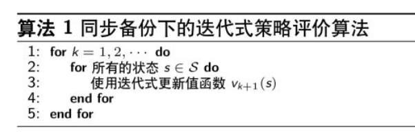
一次迭代内，状态 \(s\) 的价值等于前一次迭代该状态的即时奖励与 \(s\) 下一个所有可能状态 \(s’\) 的价值与其概率乘积的和

Policy Iteration

How to Improve a Policy

• Given a policy \(\pi\)
  • Evaluate the policy \(\pi\)
  • \(v_\pi (s) = \mathbb{E} [R_{t+1} + \gamma R_{t+2} + \cdots \mid S_t = s])
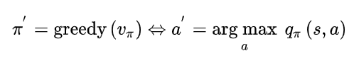
  • Improve the policy by acting greedily with respect to \(v_\pi\)
  • \(\pi’=greedy(v_\pi))

This process of policy iteration always converges to \(\pi*\).

通常来说，我们需要更多的估计/改进迭代。 尽管如此，我们的策略迭代方法总能收敛到最优策略\(\pi_*\)。

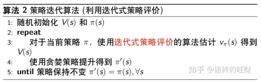
Policy Iteration

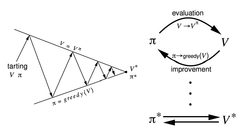
Policy evaluation: Estimate \(v_pi\); Iterative policy evaluation. Policy improvement: Generate \(\pi’ \geq \pi\); Greedy policy improvement.

Policy Improvement

We consider a deterministic policy, \(a = \pi(s)\). We can improve the policy by acting greedily:

This improves the value from any state \(s\) over one step,

It therefore improves the value function, \(v_\pi’(s) \geq v_\pi (s)\).

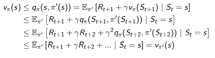
If improvements stop:

Then the Bellman optimality equation has been satisfied:

Therefore \(v_\pi (s) = v_*(s) \forall s \in \mathcal{S}\). \(\pi\) is an optimal policy.

本质上就是使用当前策略产生新的样本，然后使用新的样本更好的估计策略的价值，然后利用策略的价值更新策略，然后不断反复。 理论可以证明最终策略将收敛到最优。

Modified Policy Iteration

Does policy evaluation need to converge to \(v_\pi\)? Or should we introduce a stopping condition, such as \(\epsilon-\)convergence of value function; Or simply stop after \(k\) iterations of iterative policy evaluation?

Generalized Policy Iteration

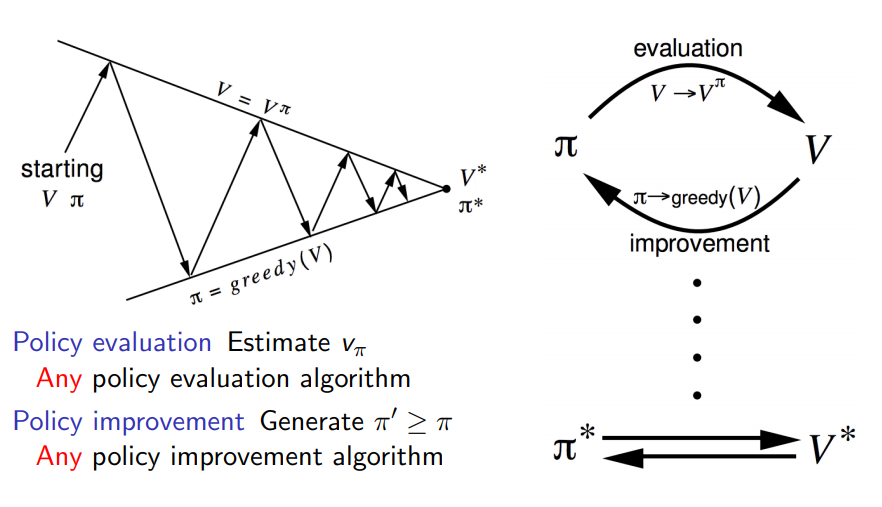
策略迭代包括两个同时进行的交互过程 一个使得值函数（value function）与当前策略一致（策略评价 policy evaluation） 另一个使得策略相对于当前值函数较贪婪（策略提升 policy improvement）。 广义策略迭代（GPI）来指代让策略评价和策略提升交互的一般概念，而不依赖于两个过程的粒度和其他细节。 几乎所有强化学习方法都可以被很好地描述为GPI。 策略总是相对于值函数被改善 并且值函数总是趋向策略下的值函数

Value Iteration

Principle of Optimality

Any optimal policy can be subdivided into two components:

• An optimal first action \(A_*\)
• Followed by an optimal policy from successor state \(s’\)

Principle of Optimality: A policy \(\pi (a \mid s)\) achieves the optimal value from state \(s\), \(v_\pi (s) = v_*(s)\), if and only if:

• For any state \(s’\) reachable from \(s\)
• \(\pi\) achieves the optimal value from state \(s’\), \(v_\pi(s’) = v_*(s’)\)

Deterministic Value Iteration

If we know the solution to subproblems \(v_(s’)\), then solution \(v_(s)\) can be found by one-step lookahead:

The idea of value iteration is to apply these updates iteratively. The intuition is to start with final rewards and work backwards.

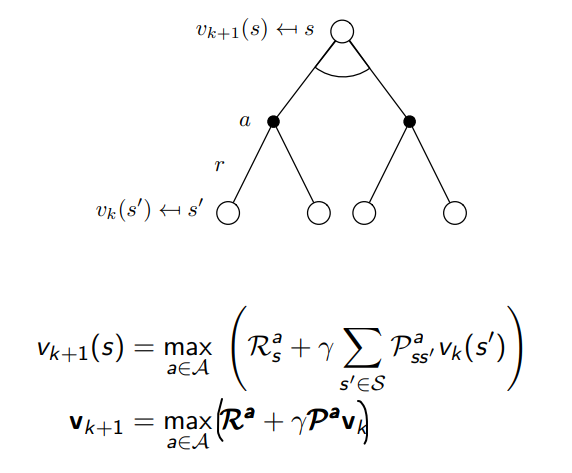
Value Iteration

• Problem: find optimal policy \(\pi\)
• Solution: iterative application of Bellman optimality backup
• \(v_1 \rightarrow v_2 \rightarrow \cdots → v_∗\)
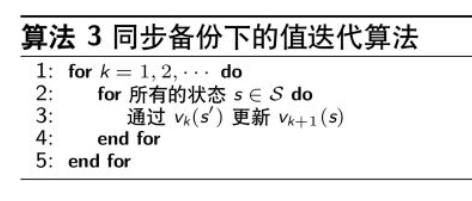
• Using synchronous backups
  • At each iteration \(k+1\)
  • For all states \(s \in \mathcal{S}\)
  • Update \(v_{k+1}(s)\) from \(v_k(s’)\)
• Unlike policy iteration, there is no explicit policy
• Intermediate value functions may not correspond to any policy

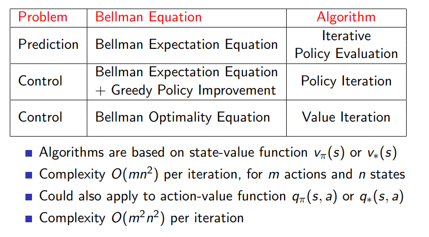
Summary of DP Algorithm

Synchronous Dynamic Programming Algorithm

Extensions to Dynamic Programming

Asynchronous Dynamic Programming

• Previous
  A Brief Survey of Deep Reinforcement Learning
• Next
  David Silver - Reinforcement Learning Note 4