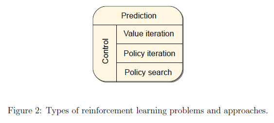
Overview
There are two key ideas that allow RL algorithms to achieve this goal:
- Use samples to compactly represent the dynamics of the control problem
- it allows one to deal with learning scenarios when the dynamics is unknown
- even if the dynamics is available, exact reasoning that uses it might be intractable on its own
- to use powerful function approximation methods to compactly represent value functions.
- it allows dealing with large, high-dimensional state and action spaces.
Markov Decision Processes
Preliminaries
\(\mathbb{N}\) denotes the set of natural numbers, while \(\mathbb{R}\) denotes the set of reals. A vector \(v\) means a column vctor.
The inner product of two finite-dimensional vectors, \(u, v \in \mathbb{R}^d\) is \(\left< u, v \right> = \sum_{i=1}^d u_i v_i\).
For a function \(f:\mathcal{x} \rightarrow \mathbb{R}\), \(\parallel \cdot \parallel_{\infty}\) is defined by \(\parallel f \parallel_{\infty}=sup_{x\in\mathcal{X}} \mid f(x) \mid \).
A mapping \(T\) between the metric space \((M_1, d_1), (M_2, d_2)\) is called Lipschitz with modulus \(L \in \mathbb{R}\) if for any \(a, b \in M_1, d_2(T(a), T(b)) \leq L d_1(a, b)\). If \(T\) is Lipschitz with a modulus \(L \leq 1\), it is called a non-expansion. If \(L < 1\), the mapping is called a contraction.
The indicator function of event \(S\) will be denoted by \(\mathbb{I}_{{S}}\), if \(S\) holds it is 1 and \(S\) not, otherwise.
If \(v = v(\theta, x), \frac{\partial}{\partial \theta}v\) shall denote the partial derivate of \(v\) with respect to \(\theta\).
If \(P\) is a distribution or a probability measure, then \(X ~ P\) means that \(X\) is a random variable drawn from \(P\).
Markov Decision Processes
A countable MDP is defined as a triplet \(\mathcal{M} = (\mathcal{X}, \mathcal{A}, \mathcal{P}_0)\), where \(\mathcal{X}\) is the countable non-empty set of states, \(\mathcal{A}\) is the countable non-empty set of actions.
The transition probability kernel \(mathcal{P}_0\) assigns to each state-action pair \((x, a) \in \mathcal{X} \times \mathcal{A}\) a probability measure over \(\mathcal{X} \times \mathbb{R}\), which we shall denote by \(\mathcal{P}_0 (\cdot \mid x, a)\). For \(U \subset \mathcal{X} \times \mathbb{R}\), \(\mathcal{P}_0(U \mid x, a)\) gives the probability that the next state and the associated reward belongs to the set \(U\) provided that the current state is \(x\) and the action taken is \(a\).
Transition Probability Kernel 转移概率核是一个二元组(state, reward)
The state transition probability kernel, \(\mathcal{P}\), which for any \((x, a, y) \in \mathcal{X} \times \mathcal{A} \times \mathcal{X}\) triplet gives the probability of moving from state \(x\) to some other state \(y\) provided that action a was chosen in state \(x\):
\[\mathcal{P}(x, a, y) = \mathcal{P}_0(\{y\} \times \mathbb{R} \mid x, a)\]State transition probability kernel 状态转移概率核P在输入为(x, a, y)时,代表从状态x,通过动作a,转移到状态y的概率
They also give rise to the immediate reward function \(r\): \(\mathcal{X} \times \mathcal{A} \rightarrow \mathbb{R}\), which gives the expected immediate reward received when action \(a\) is chosen in state \(x\): if \((Y_{(x,a)}, R_{(x,a)}) ~ \mathcal{P}_0(\cdot \mid x, a)\), then
\[r(x,a) = \mathbb{E}[R_{(x,a)}]\]immediate reward function 即时奖励函数是指在状态x下采取动作a之后获得奖励的期望
An MDP is called finite if both \(\mathcal{X}, \mathcal{A}\) are finite.
Markov Decision Processes are a tool for modeling sequential decision-making problems where a decision maker interacts with a system in a sequential fashion.
Given an MDP \(\mathcal{M}\), let \(t \in \mathbb{N}\) denote the current time stage, let \(X_t \in \mathcal{X}\) and \(A_t \in \mathcal{A}\) denote the random state of the system and the action chosen by the decision maker at time \(t\). Once the action is selected, it is sent to the system, which make a transition:
\[(X_{t+1}, R_{t+1}) ~ \mathcal{P}_0(\cdot \mid X_t, A_t)\]\(X_{t+1}\) is random and \(\mathbb{P}(X_{t+1} = y \mid X_t = x, A_t = a)= \mathcal{P}(x, a, y)\). \(\mathbb{E}[R_{t+1} \mid X_t, A_t] = r(X_t, A_t)\). The decision maker then observes the next state \(X_{t+1}\) and reward \(R_{t+1}\), chooses a new action \(A_{t+1} \in A\) and the process is repeated.
The goal of the decision maker is to come up with a way of choosing the actions so as to maximize the expected total discounted reward.
A rule describing the way the actions are selected is called a behavior.
History sequence: \(X_0, A_0, R_1, \cdots, X_{t-1}, A_{t-1}, R_{t}, X_{t}\).
The return underline a behavior is defined as the total discounted sum of the rewards incurred:
\[\mathcal{R} = \sum_{t=0}^\infty \gamma^t R_{t+1}\]If \(\gamma < 1\) then rewards far in the future worth exponentially less than the reward received at the first stage. It is called a discounted reward MDP, while undiscounted when \(\gamma = 1\).
The goals of the decision-maker is to choose a behavior that maximizes the expected return, such a maximizing behavior is said to be optimal.
样例一:库存控制
库存大小一定,每日需求不确定:每晚都需要决定明天需要的订货量,早晨会送货来填充库存。白天会根据需求量情调库存,需求量是以一个固定分布独立的。
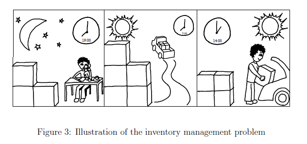
仓储主观的目标是是管理库存,以便以使预期的未来总收入的现值最大化。
在时间步骤 \(t\) 定义为:对于每次购买 \(A_t\),物品价格为 \(K \mathbb{I}_{A_t>0} + cA_t\)。也就是说,对于每次购买都有一个固定支出\(K\),每件购买的货物按照一个固定的价格 \(c\),且 \(K, c >0\)。另外,当货物持有 \(x>0\)时也有一个仓储成本,简单来说这个成本以\(h>0\)正比于仓库大小。最后,售出 \(z\)单位的货物后,可以获得 \(pz\)的收入,其中 \(p>0\)。当然,\(p>h\) 才可以使得我们获取利润。
这儿问题可以表示成为一个MDP:令 \(X_t\) 为第 \(t\) 天晚上的库存量,\(\mathcal{X} = {0, 1, \cdots, M}\),\(M\)为最大仓储量。动作 \(A_t\) 为当天晚上的订货量。因此,我们的动作区间为 \(\mathcal{A} = {0, 1, \cdots, M}\),我们无需考虑货物大于仓储量的状态。一旦给定,我们可以得到第二天的状态:
\[X_{t+1} = ((X_t + A_t) \wedge M - D_{t+1})^+\]我们将 \(\wedge\)符号定义为求最小值,而\(\ ^+\) 定义为与零求最大值。 \(D_{t+1} \in \mathbb{N}\)为下一天的需求量。根据假设,需求量是一系列独立且分布均匀的整数值随机变量。因此,我们对于第 \(t+1\)天的利润可以写为:
\[R_{t+1} = -K \mathbb{I}_{\{A_t > 0\}} - c((X_t + A_t) \wedge M - X_t)^+ - h X_t + p((X_t + A_t) \wedge M - X_{t+1})^+\]利润首先先扣除 \(t\) 天购买的花费(最多不能超过M),扣除\(t\)天的仓储成本,最后加上 \(t+1\) 天的收入。以上两个式子可以写成紧凑的形式:
\[(X_{t+1}, R_{t+1}) = f(X_t, A_t, D_{t+1})\]我们可以得到 \(\mathcal{P}\):
\[\mathcal{P}_0(U \mid x, a) = \mathbb{P}(f(x, a, D) \in U) = \sum_{d=0}^\infty \mathbb{I}_{\{f(x, a, d) \in U\}p_D}(d)\]其中 \(p_D(\cdots)\) 是随机需求的概率质量函数,并且 \(D ~ p_D(\cdot)\)。
In some MDPs, some states are impossible to leave, no matter what actions are selected after time \(t\). By convention, we will assume that no reward is incurred in such terminal or absorbing states. An MDP with such states is called episodic. An episode then is the time period from the beginning of time until a terminal state is reached. In an episodic MDP, we often consider undiscounted rewards, \(\gamma = 1\).
赌徒问题
一个赌徒进入游戏,他可以拿财产 \(X_t \geq 0\) 中的任意比例 \(A_t \in [0, 1]\)赌博,并且以 \(p \in [0, 1] \) 的概率赢回赌注或者赚的更多,也有可能以 \(1-p\) 输掉赌注。因此,赌徒的财产可以表示为:
\[X_{t+1} = X_t + S_{t+1}A_t X_t = (1 + S_{t+1}A_t) X_t\]其中,\(S_t\) 是一系列取值为\({-1, +1}\)的独立变量,乘以概率分布 \(\mathbb{P}(S_{t+1}=1)=p\)。赌徒的目的肯定是最大化他的财富,设一个峰值为 \(w* >0\)。初始财富介于 \([0, w*]\)之间。
我们可以把这个问题转换为片段MDP问题,状态空间为\(\mathcal{X}=[0, w*]\),动作空间为 \(\mathcal{A} = [0, 1]\)。我们定义:
\[X_{t+1} = (1 + S_{t+1}A_t)X_t \wedge w*\]我们将 \(w\) 设为一个终止状态: \(X_{t+1} = X_t\) if \(X_t=w\)。只要不达到状态 \(X_{t+1} < w*\),即时收益为0,否则第一次到达状态则为1。
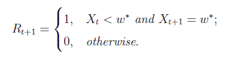
如果将折扣系数设置为1,则根据财富是否达到\(w*\),沿任何轨迹的总奖励将为1或0。 因此,预期的总奖励仅仅是赌徒的财富达到w的概率。
In practical applications, the state- and action-spaces are often very large, multidimensional space.
Value Functions
A better approach of finding an optimal behavior in some MDP is based on computing value functions. In this approach, one first computes the so-called optimal value function.
The optimal value, \(V(x)\), of state \(x \in \mathcal{X}\) gives the highest achievable expected return when the process is started from state \(x\). The function \(V: \mathcal{X} \rightarrow \mathbb{R}\) is called the optimal value function. A behavior that achieves the optimal values in all states is optimal.
Deterministic stationary policies represent a special class of behaviors, which play an important role in the theory of MDPs. They are specified by some mapping \(\pi\), which map states to actions, such as \(\pi: \mathcal{X} \rightarrow \mathcal{A}\). Following \(\pi\) means that at any time \(t \geq 0\) the action \(A_t\) is selected using
\[A_t = \pi(X_t)\]A stochastic stationary policy \(\pi\) maps states to distributions over the action space. We shall use \(\pi(a \mid x)\) to denote the probability of action \(a\) being selected by \(\pi\) in state \(x\). If a stationary policy is followed in an MDP, if:
\[A_t ~ \pi(\cdot \mid X_t), t\in \mathbb{N}\]the state process will be a Markov chain.
A stationary policy and and MDP induce what is called a Markov Reward Processes (MRP): an MRP is determined by the pair \(\mathcal{M}=(\mathcal{X}, \mathcal{P}_0)\), where now \(\mathcal{P}_0\) assigns a probability measure over \(\mathcal{X} \times \mathbb{R}\) to each state.
An MRP \(\mathcal{M}\) gives rise to the stochastic process, where \(X_{t+1}, R_{t+1} ~ \mathcal{P}_0(\cdot \mid X_t)\).
The value function, \(V^\pi: \mathcal{X} \rightarrow \mathbb{R}\), underlying \(\pi\) is defined by:
\[V^\pi(x) = \mathbb{E} [\sum_{t=0}^\infty \gamma^t R_{t+1} \mid X_0 = x], x \in \mathcal{X}\]with the understanding that:
- the process is the reward \(R_t\) part of the process \((X_t, A_t, R_{t+1})\) obtained when following policy \(\pi\)
- \(X_0\) is selected at random such that \(\mathbb{P}(X_0=x)>0\) holds for all states \(x\). For MRP, it is defined as:
It will also be useful to define the action-value function, \(Q^\pi: \mathcal{X} \times \mathcal{A} \rightarrow \mathbb{R}\), underlying a policy \(\pi\) in an MDP. Let \((X_t, A_t, R_{t+1})\) be the resulting stochastic process, then:
\[Q^\pi(x,a) = \mathbb{E}[\sum_{t=0}^\infty \gamma^t R_{t+1} \mid X_0=x, A_0 = a], x \in \mathcal{X}, a \in \mathcal{A}\]The optimal value- and action-value functions are connected by the following equations:
\[V*(x) = \sup _{a\in \mathcal{A}} Q*(x, a), x \in \mathcal{X}\] \[Q*(x, a) = r(x, a) + \gamma \sum_{y \in \mathcal{X}} \mathcal{P}(x, a, y) V*(y), x \in \mathcal{X}, a \in \mathcal{A}\]In the class of MDPs, an optimal stationary policy always exists:
\[V*(x) = \sum_{\pi} V^\pi(x), x \in \mathcal{X}\] \[\sum_{a\in A} \pi (a\mid x) Q*(x, a) = V*(x)\]An action that maximizes \(Q(x, \cdot)\) is called greedy with respect to \(Q\) in state \(x\). A greedy policy with respect to \(Q*\) is optimal.
The next question is how to find \(V\) or \(Q\), how to find the value function of a policy:
Bellman Equations for Deterministic Policy: Fix an MDP \(\mathcal{M} = (\mathcal{X}, \mathcal{A}, \mathcal{P}_0)\), a discount factor \(\gamma\) and deterministic policy \(\pi\). Let \(r\) be the immediate reward function of \(\mathcal{M}\). Then \(V^\pi\) satisfies:
\[V^\pi (x) = r(x, \pi(x)) + \gamma \sum_{y \in \mathcal{X}} \mathcal{P}(x, a, y) V^\pi(y), x \in \mathcal{X}\]Define the Bellman operator underlying \(\pi, T^\pi: \mathbb{R}^\mathcal{X} \rightarrow \mathbb{R}^\mathcal{X}\) by:
\[(T^\pi V)(x) = r(x, \pi(x)) + \gamma \sum_{y \in \mathcal{X}} \mathcal{P}(x, a, y) V(y), x \in \mathcal{X}\]When the state space \(\mathcal{X}\) is finite, it has \(D\) states, \(\mathbb{R}^\mathcal{X}\) can be identified with the \(D\)-dimensional Euclidean space and \(V \in \mathbb{R}^\mathcal{X}\) can be thought of as a \(D\)-dimensional vector. In this case, it can be written in the form:
\[r^\pi + \gamma P^\pi V\pi = V\pi\]The optimal value function is known to satisfy a certain fixed-point equation:
\[V*(x) = (T*V)(x) = \sup{a\in \mathcal{A}}{r(x,a) + \gamma \sum_{y \in \mathcal{X}}\mathcal{P}(x,a,y)V(y)}, x \in \mathcal{X}\]If \(0 < \gamma < 1\), then \(T\) is a maximum-norm contraction, and the fixed-point equation \(TV = V\) has a unique solution.
The action-value function underlying a policy and the optimal action-value function also satisfy some fixed point equations similar to the previous ones:
\(T\pi Q(x,a) = r(x,a) + \gamma \sum_{y\in \mathcal{X}}\mathcal{P}(x,a,y)Q(y, \pi(y)), (x,a) \in \mathcal{X} \times \mathcal{A}\) \(T* Q(x,a) = r(x,a) + \gamma \sum_{y\in \mathcal{X}}\mathcal{P}(x,a,y)\sup{a' \in \mathcal{A}}Q(y, a'), (x,a) \in \mathcal{X} \times \mathcal{A}\)
Note that \(T\pi\) is affine linear, \(T*\) is nonlinear.
The action-value function of \(\pi, Q^\pi\), satisfies \(T^\pi Q^\pi = Q^\pi\) and \(Q\pi\) is the unique solution to this fixed-point equation.
Dynamic Programming Algorithms for solving MDPs
Value iteration generates a sequence of value functions:
\[V_{k+1} = T*V_k, k \geq 0\]where \(V_0\) is arbitrary. \(V_k\) converges to \(V*\) at a geometric rate.
Value iteration can also be used in conjunction with action-value functions; in which case, it takes the form:
\[Q_{k+1} = T*Q_k, k \geq 0\]which again converges to \(Q\) at a geometric rate. The idea is that once \(V_k\) (or \(Q_k\)) is close to \(V\) (or \(Q*\)), a policy that is greedy with respect to \(V_k\) (or \(Q_k\)) will be close to optimal.
Policy iteration works as follows. Fix an arbitrary initial policy \(\pi_0\). At iteration \(k > 0\), compute the action-value function underlying \(\pi_k\). Next, given \(Q^{\pi_k}\), define \(\pi_{k+1}\) as a policy that is greedy with respect to \(Q^{\pi_k}\). After \(k\) iterations, policy iteration gives a policy not worse than the policy that is greedy to the value function computed using \(k\) iterations of value iteration if the two procedures are started with the same initial value function. However, the computational cost of a single step in policy iteration is much higher than that of one update in value iteration.