Value prediction problems arise in a number of ways:
- Estimating the probability of some future event
- The expected time until some event occurs
- The (action-) value function underlying some policy in an MDP
Since the value of a state is defined as the expectation of the random return when the process is started from the given state, an obvious way of estimating this value is to compute an average over multiple independent realizations started from the given state. This is an instance of Mente-Carlo method.
The variance of the Mente-Carlo returns can be high, which means that the quality of the estimates will be poor. When interacting with a system in a closed-loop fashion, it might be impossible to reset the state of the system to some particular state. In this case, the Monte-Carlo technique cannot be applied without introducing some additional bias.
Temporal difference (TD) learning which is without doubt one of the most significant ideas in reinforcement learning, is a method that can be used to address these issues.
Temporal difference learning in finite state spaces
The unique feature of TD learning is that it uses bootstrapping: predictions are used as targets during the course of learning.
Tabular TD(0)
Fix some finite Markov Reward Process \(\mathcal{M}\). We wish to estimate the value function \(V\) underlying \(\mathcal{M}\) given a realization \((X_t, R_{t+1})\). Let \(\hat{V}_t(x)\) denote the estimate of state \(x\) at time \(t\). In the \(t^{th}\) step TD(0) performs the following calculations:
\[\delta_{t+1} = R_{t+1} + \gamma \hat{V}_t(X_{t+1}) - \hat{V}_t(X_t)\] \[\hat{V}_{t+1}(x) = \hat{V}_t(x) + \alpha_t \delta_{t+1} \mathbb{I}_{\{X_t = x\}}, x \in \mathcal{X}\]Here the step-size sequence \(\alpha_t\) consists of small nonnegtive numbers chosen by the user.
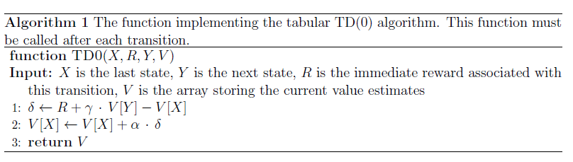
The only value changed is the one associated with \(X_t\). When \(\alpha \leq 1\), the value of \(X_t\) is moved towards the “target” \(R_{t+1} + \gamma \hat{V}t(X{t+1})\). Since the target depends on the estimated value function, the algorithm use bootstrapping.
The term “temporal difference” comes from that \(\delta_{t+1}\) is defined as the difference between values of states corresponding to successive time steps. \(\delta_{t+1}\) is called a temporal difference error.
TD(0) is a stochastic approximation algorithm. If it converges, then it must converge to a function \(\hat{V}\) such that the expected temporal difference given \(\hat{V}\):
\[F \hat{V} (x) \overset{def}{=} \mathbb{E} [R_{t+1} + \gamma \hat{V}(X_{t+1}) - \hat{V}(X_t) \mid X_t = x]\]is zero at least for all states that are sampled infinitely often.
A simple calculation shows that \(F \hat{V} = T \hat{V} - \hat{V}\), where \(T\) is the Bellman-operator underlying the MRP considered. \(F \hat{V} = 0\) has a unique solution. Thus, if TD(0) converges then it must converge to \(V\).
For simplicity, assume that \(X_t\) is a stationary, ergodic Markov chain. Identify the approximate value function \(\hat{V}_t\) with D-dimensional vectors. Then, assuming that the step-size sequence satisfies the Robbins-Monoro (RM) conditions:
\[\sum_{t=0}^{\infty} \alpha_t = \infty, \sum_{t=0}^{\infty} \alpha_t^2 < +\infty\]The sequence \(\hat{V}_t\) will track the trajectories of the ordinary differential equation:
\[\dot{v}(t) = cF(v(t))\]where \(c = \frac{1}{D}\) and \(v(t) \in \mathbb{R}^D\). The above (linear) ODE can be written as
\[\dot{v} = r + (\gamma P - I)v\]Since the eigenvalues of \(\gamma P - I\) all lie in the open left half complex plane, this ODE is globally asymptotically stable. Using standard results of SA it follows that \(\hat{V}_t\) converges almost surely to V.
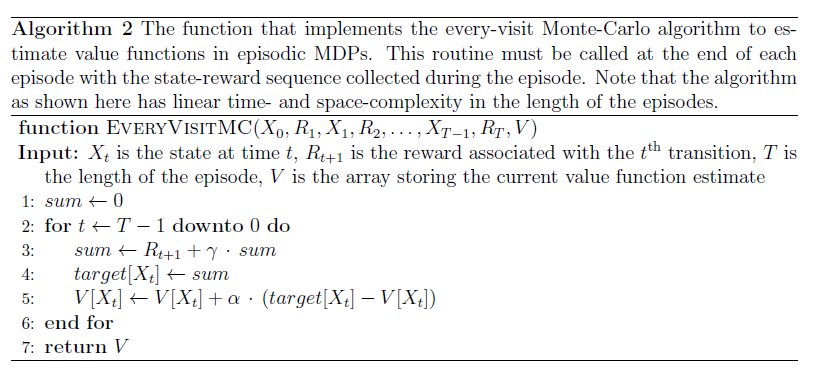
Every-visit Monte-Carlo
Consider some episodic problem. Let the uderlying MRP be \(\mathcal{M} = (\mathcal{X}, \mathcal{P}0)\) and let \((X_t, R{t+1}, Y_{t+1})\) be generated by continual sampling in \(\mathcal{M}\) with restarts from some distribution \(\mathcal{P}0\) defined over \(\mathcal{X}\). Let \(T_k\) be the sequence of times when an eisode starts. For a given time \(t\), let \(k(t)\) be the unique episode index such that \(t \in [T_k, T{k+1}]\). Let:
\[\mathcal{R}_t = \sum_{s=t}^{T_{k(t) + 1}-1} \gamma^{s-t} R_{s+1}\]denote the return from time \(t\) on until the end of the episode. \(V(x) = \mathbb{E} [\mathcal{R}_t \mid X_t = x]\) for any state \(x\) such that \(\mathbb{P}(X_t = x) >0\). A sensible ways of updating the estimates is to use:
\[\hat{V}_{t+1}(x) = \hat{V}_t(x) + \alpha_t(\mathcal{R}_t - \hat{V}_t(x)) \mathbb{I}_{\{X_t = x\}}, x \in \mathcal{X}\]Monte-Carlo methods such as the above one, since they use multi-step prediction of the value, are called multi-step methods.
This algorithm is again an instance of stochastic approximation.
TD(0) or Monte-Carlo
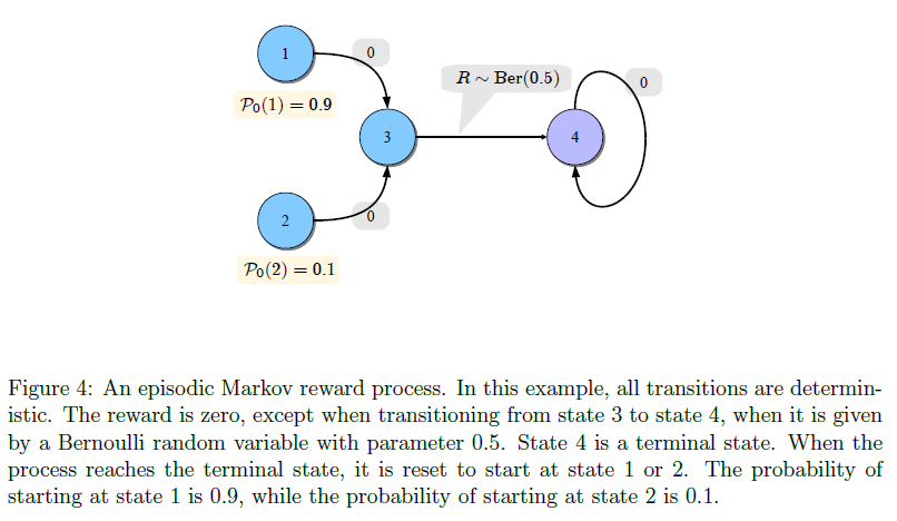
Consider the undiscounted episodic MRP shown above. The initial states are either 1 or 2. Consider now how TD(0) will behave at state 2. By the time state 2 is visited the \(k^{th}\) time, on the average state 3 has already been visited \(10k\) times. Assume that \(\alpha_t = 1 / (t+1)\). At state 3 the TD(0) update reduces to averaging the Bernoulli rewards incurred upon leaving state 3.
At the \(k^{th}\) visit of state 2, \(Var[\hat{V}_t(3)] \approx 1/(10k)\), \(\mathbb{E}[\hat{V}_t(3)] = V(3) = 0.5\). Thus, the target of the update of state 2 will be an estimate of the true value of state 2 with accuracy increasing with \(k\).
Now consider the Monte-Carlo method. This method ignores the estimate of the value of state 3 and uses the Bernoulli reward directly. In particular, \(Var[R_t \mid X_t = 2] = 0.25\). On this example, this makes the Monte-Carlo method slower to converge, showing that sometimes bootstrapping might indeed help.
Another example when bootstrapping is not helpful. Imagine that the problem is modified so that the reward associated with the transition from state 3 to state 4 is made deterministically equal to 1. The Monte-Carlo method becomes faster since \(R_t = 1\) is the true target value, while for the value of state 2 to get close to its true value, TD(0) has to wait until the estimate of the value at state 3 becomes close to its true value. This slows down the convergence of TD(0).
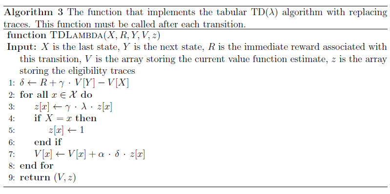
TD(λ): Unifying Monte-Carlo and TD(0)
Here, \(\lambda \in [0, 1]\) is a parameter that allows one to interpolate between the Monte-Carlo and TD(0) updates: \(\lambda = 0\) gives TD(0), while \(\lambda = 1\), TD(1) is equivalent to Monte-Carlo method.
In essence, given some \(\lambda > 0\), the targets in the TD(λ) update are given as some mixture of the multi-step return predictions:
\[\mathcal{R}_{t:k} = \sum_{s=t}^{t+k} \gamma ^{s-t} R_{s+1} + \gamma^{k+1} \hat{V}_t (X_{t+k+1})\]where the mixing coefficients are the exponential weights weights \((1-\lambda)\lambda^k\). Thus, for \(\lambda >0\), TD(λ) will be a multi-step method. The algorithm is made incremental by the introduction of the so-called eligibility trace.
In fact, the eligibility traces can be defined in multiple ways and hence TD(λ) exists in correspondingly many multiple forms. The update rule of TD(λ) with the so-called accumulating traces is as follows:
\[\delta_{t+1} == R_{t+1} + \gamma \hat{V}_t(X_{t+1}) - \hat{V}_t(X_t)\\ z_{t+1}(x) = \mathbb{I}_{\{x = X_t\}} + \gamma \lambda z_t(x)\\ \hat{V}_{t+1}(x) = \hat{V}_t(x) + \alpha_t \delta_{t+1} z_{t+1}(x)\\ z_0(x) = 0, x \in \mathcal{X}\]Here \(z_t(x)\) is the eligibility trace of state x. In these updates, the trace-decay parameter λ controls the amount of bootstrapping.
Replacing traces and \(\lambda = 1\) correspond to a version of the Monte-Carlo algorithm where a state is updated only when it is encountered for the first time in a trajectory. The corresponding algorithm is called fi rst-visit Monte-Carlo method.
In summary, TD(λ) allows one to estimate value functions in MRPs. It generalizes Monte-Carlo methods, it can be used in non-episodic problems, and it allows for bootstrapping. Further, by appropriately tuning λ it can converge significantly faster than Monte-Carlo methods or TD(0).