A catalog of learning problems
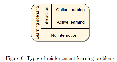
The first criterion that the space of problems is split upon is whether the learner can actively influence the observations. In case it can, then we talk about interactive learning, otherwise one is facing a non-interactive learning problem.
Interactive learning is potentially easier since the learner has the additional option to influence the distribution of the sample.
In the case of non-interactive learning, the natural goal is to find a good policy given the observations. A common situation is when the sample is fixed. In machine learning terms, this corresponds to batch learning. Since the observations are uncontrolled the learner working with a fixed sample has to deal with an off-policy learning situation.
In other cases, the learner can ask for more data. Here the goal might be to learn a good policy as quickly as possible.
Now consider interactive learning. One possibility is that learning happens while interacting with a real system in a closed-loop fashion. A reasonable goal then is to optimize online performance, making the learning problem an instance of online learning.
Online performance can be measured in different ways. A natural measure is to use the sum of rewards incurred during learning. An alternative cost measure is the number of times the learner’s future expected return falls short of the optimal return. Another possible goal is to produce a well-performing policy as soon as possible, just like in non-interactive learning.
As opposed to the non-interactive situation, however, here the learner has the option to control the samples so as to maximize the chance of finding such a good policy. This learning problem is an instance of active learning.
Closed-loop Interactive Learning
The special feature of interactive learning is the need to explore.
Online Learning in Bandits
Consider an MDp that has a single state. Let the problem be that of maximizing the reutrn while learning. Since there is only one state, this is an instance of the classical bandit problems. A basic observation is that a bandit learner who always chooses the action with the best estimated payoff can fail to find the best action with positive probability, which in turn leads to a large loss. Thus, a good learner must take actions that look suboptimal, must explore. The question is then how to balance the frequency of exploring and exploiting actions.
A simple strategy is to fix \(\epsilon > 0\) and choose a randomly selected action with probability ε, and go with the greedy choise otherwise. This is called ε-greedy strategy. Another simple strategy is the so-called “Boltzmann exploration” strategy. Given the sample means, \((Q_t(a); a\ in \mathcal{A})\), of the action at time \(t\), the next action is drawn from the multinomial distribution \((\pi(a); a \in \mathcal{A})\), where
\[\pi (a) = \frac{\exp (\beta Q_t(a))}{\sum_{a' \in A} \exp (\beta Q_t(a'))}\]Here \(\beta > 0\) controls the greediness of action selection. The difference between Bolzmann exploration and ε-greedy is that ε-greedy does not take into account the relative values of the actions, while Boltzmann exploration does. These algorithms extend easily to the case of unrestricted MDPs provided that some estimates of te action-values in available.
If the parameter of ε-greedy is made a function of time and the resulting sequence is appropriately tuned, ε-greedy can be made competitive with others. However, the best choice is problem dependent and there is no known automated way of obtaining good results with ε-greedy.
A better approach might be to implement the so-called optimism in the face of uncertainty (OFU) principle, according to which the learner should choose the action with the best upper confidence bound (UCB). UCB1 implements this principle by assigning the following UCB to action \(a\) at time \(t\):
\[U_t(a) = r_t(a) + \mathcal{R}\sqrt(\frac{2 \log t}{n_t(a)})\]Here \(n_t(a)\) is the number of times \(t\) and \(r_t(a)\) is the sample mean of the \(n_t(a)\) rewards observed for action \(a\), whose range is \([-\mathcal{R}, \mathcal{R}]\). It can be shown that the failure probability of \(U_t(a)\) is \(t^{-4}\).
Notice that an action’s UCB is lager if less information is available for it. An action’s UCB value increases even if it is not tried.
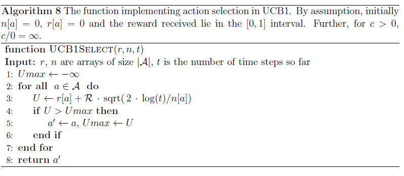
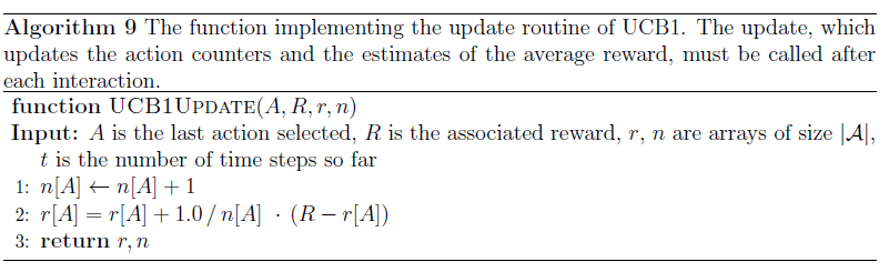
Algorithms above show the pseudocode of UCB1, in the form of two routines, one to be used for action selection and the other for updating the internal statistics.
When the variance of the rewards associated with some of the actions are small, it makes sense to estimate these variances and use them in place of the range \(\mathcal{R}\) in the above algorithm.
The setting considered here is called the frequentist agnostic setting, where the only assumption made about the distribution of rewards is that they are independent across the actions and time steps and that they belong to the \([0, 1]\) interval. However, there is no other a priori knowledge about their distributions.
An alternative, historically significant, variant of the problem is when the reward distributions have some known parametric form and the parameters are assumed to be drawn from a known prior distribution. The problem then is to find a policy which maximizes the total expected cumulated discounted reward, where the expectation is both over the random rewards and the parameters of their distributions.
This problem can be represented as an MDP whose state at time \(t\) is the posterior over the parameters of the reward distributions.
The conceptual difficulty of this so-called Bayesian approach is that although the policy is optimal on the average for a collection of randomly chosen environments, there is no guarantee that the policy will perform well on the individual environments. The appeal of the Bayesian approach, however, is that it is conceptually very simple and the exploration problem is reduced to a computational problem.
Active Learning in Bandits
Let the goal be to find an action with the highest immediate reward given \(T\) interactions. Since the rewards received during the course of interaction do not matter, the only reason not to try an action is if it can be seen to be worse than some other action with sufficient certainty. The remaining actions should be tried in the hope of proving that some are suboptimal. A simple way to achieve this is to compute upper and lower confidence bounds for each action:
\[U_t(a) = Q_t(a) + \mathcal{R}\sqrt{\frac{\log (2 \mid \mathcal{A} \mid T / \delta)}{2t}}\\ U_t(a) = Q_t(a) - \mathcal{R}\sqrt{\frac{\log (2 \mid \mathcal{A} \mid T / \delta)}{2t}}\]and eliminate an action \(a\) if \(U_t(a) < )