Graph Convolutional Policy Network for Goal-Directed Molecular Graph Generation

Graph Convolutional Policy Network for Goal-Directed Molecular Graph Generation

Generating novel graph structures that optimize given objectives while obeying some given underlying rules is fundamental for chemistry and biology. However, designing models to find molecules that optimize desired properties while incorporating highly complex and non-differentiable rules remains to be a challenging task. Graph Convolutional Policy Network (GCPN), a general graph convolutional network based model for goal-directed graph generation through reinforcement learning. The model is trained to optimize domain-specific rewards and adversarial loss through policy gradient, and acts in an environment that incorporates domain-specific rules.

The generation of novel and valid molecular graphs that can directly optimize various desired physical, chemical and biological property objectives remains to be a challenging task, since these property objectives are highly complex and non-differentiable.

GCPN is an approach to generate molecules where the generation process can be guided towards specified desired objectives, while restricting the output space based on underlying chemical rules. The entire model is trained end-to-end in the reinforcement learning framework. A reinforcement learning approach has several advantages compared to learning a generative model over a dataset. Firstly, desired molecular properties and molecule constraints are complex and non-differentiable, thus they cannot be directly incorporated into the objective function of graph generative models. In contrast, reinforcement learning is capable of directly representing hard constraints and desired properties through the design of environment dynamics and reward function. Secondly, reinforcement learning allows active exploration of the molecule space beyond samples in a dataset.

Graph representation learning is used to obtain vector representations of the state of generated graphs. We represent molecules directly as molecular graphs, which are more robust than intermediate representations such as SMILES. Partially generated molecular graphs can be interpreted as substructures, whereas partially generated text representations in many cases are not meaningful.

Adversarial loss is used as reward to incorporate prior knowledge specified by a dataset of example molecules. Adversarial training addresses the challenge through a learnable discriminator adversarially trained with a generator.

A molecule is successively constructed by either connecting a new substructure or an atom with an existing molecular graph or adding a bond to connect existing atoms. GCPN predicts the action of the bond addition, and is trained via policy gradient to optimize a reward composed of molecular property objectives and adversarial loss. The adversarial loss is provided by a graph convolutional network based discriminator trained jointly on a dataset of example molecules.

Proposed Method

Problem Definition

We represent a graph \(G\) as \((A, E, F)\), where \(A \in {0, 1}^{n\times n}\) is the adjacency matrix, and \(F \in \mathbb{R}^{n\times d}\) is the node feature matrix assuming each node has \(d\) features. We define \(E \in {0, 1}^{b\times n\times n}\) to be the edge-conditioned adjacency tensor, assuming there are \(b\) possible edge types. \(E_{i, j, k} = 1\) if there exists an edge of type \(i\) between nodes \(j\) and \(k\), and \(A=\sum_{i=1}^b E_i\).

Our primary objective is to generate graphs that maximize a given property function \(S(G) \in \mathbb{R}\), i.e., maximize \(\mathbb{E}_{G’}[S(G’)]\), where \(G’\) is the generated graph, and \(S\) could be one or multiple domain-specific statistics of interest.

It’s also important to constrain our model with two main sources of prior knowledge:

• Generated graphs need to satisfy a set of hard constraints
• We provide the model with a set of example graphs \(G ~ p_{data}(G)\), and would like to incorporate such prior knowledge by regularizing the property optimization objective with \(\mathbb{E}_{G, G’}[J(G, G’)]\) under distance metric \(J(\cdot, \cdot)\).

Graph Generation as Markov Decision Process

We designed an iterative graph generation process and formulated it as a general decision process \(M=(\mathcal{S}, \mathcal{A}, \mathcal{P}, \mathcal{R}, \gamma)\), where \(\mathcal{S} = {s_i}\) is the set of states that consists of all possible intermediate and final graphs; \(\mathcal{A}={a_i}\) is the set of actions that describe the modification made to current graph at each time step; \(\mathcal{P} = p(s_{t+1} \mid s_t, \cdots, s_0, a_t)\) is the transition dynamics that specifies the possible outcomes of carrying out an action; \(\mathcal{R}(s_t)\) is a reward function that specices the reward after reaching state \(s_t\), and \(\gamma\) is the discount factor. The procedure to generate a graph can then be described by a trajectory \((s_0, a_0, r_0, \cdots, s_n, a_n, r_n)\), where \(s_n\) is the final generated graph. The modification of a graph at each time step can be viewed as a state transition distribution:

where \(p(a_t \mid s_t, \cdots, s_0)\) is usually represented as a policy network \(\pi_\theta\).

We design a graph generation procedure that can be formulated as a MDP, which requires the state transition dynamics to satisfy the Markov property: \(p(s_{t+1} \mid s_t, \cdots, s_0) = p(s_{t+1}) \mid s_t). Under this property, the policy network only needs the intermediate graph state \(s_t\) to derive an action. The action is used by the environment to update the intermediate graph being generated.

Molecule Generation Environment

The environment builds up a molecular graph step by step through a sequence of bond or substructure addition actions given by GCPN.

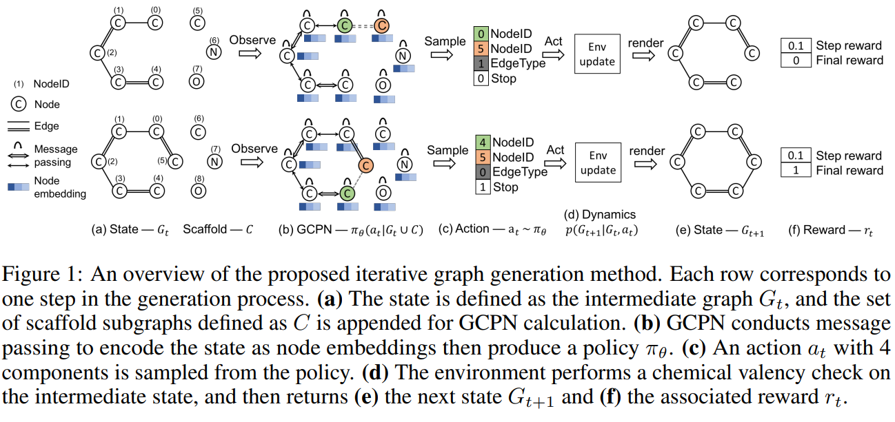
Figure 1 illustrates the 5 main components that come into play in each step, namely state representation, policy network, action, state transition dynamics and reward.

State Space: We define the state of the environment \(s_t\) as the intermediate generated graph \(G_t\) at time step \(t\), which is fully observable by the agent. Figure 1 (a) (e) depicts the partial generated molecule state before and after an action is taken. At the start of generation, we assume \(G_0\) contains a single node that represents a carbon atom.

Action Space: We define a distinct, fixed-dimension and homogeneous action space amenable to reinforcement learning. We design an action analogous to link prediction, which is a well studied realm in network science. We first define a set of scaffold subgraphs \({C_1, \cdots, C_s}\) to be added during graph generation and the collection is defined as \(C=\cup_{i=1}^s C_i\). Given a graph \(G_t\) as step \(t\), we define the corresponding extended graph as \(G_t \cup C\). Under this definition, an action can either correspond to connecting a new subgraph \(C_i\) to a node in \(G_t\) or connecting existing nodes within graph \(G_t\). Once an action is taken, the remaining disconnected scaffold subgraphs are removed.

We adopt the most fine-grained version where \(\mathcal{C}\) consists of all \(b\) different single node graphs, where \(b\) denotes the number of different atom types. Note that \(\mathcal{C}\) can be extended to contain molecule substructure scaffolds, which allows specification of preferred substructures at the cost of model flexibility.

State Transition Dynamics: Domain-specific rules are incorporated in the state transition dynamics. The environment carries out actions that obey the given rules. Infeasible actions proposed by the policy network are rejected and the state remains unchanged. For the task of molecule generation, the environment incorporates rules of chemistry. The graph-based molecular representation enables us to perform this step-wise valency check, as it can be conducted even for incomplete molecular graphs.

Reward Design: Both intermediate rewards and final rewards are used to guide the behavior of the RL agent. We define the final reward as a sum over domain-specific reward and adversarial rewards. The domain-specific rewards consist of the final property score. The intermediate rewards include step-wise validity rewards and adversarial rewards. A small positive reward is assigned if the action does not violate valency rules, otherwise a small negative reward is assigned. When the environment updates according to a terminating action, both a step reward and a final reward are given, and the generation process terminates.

To ensure that the generated molecules resemble a given set of molecules, we employ the GAN framework to define the adversarial reward \(V(\pi_\theta, D_\phi)\):

where \(\pi_\theta\) is the policy network, \(D_\phi\) is the discriminator network, x represents an input graph, \(p_data\) is the underlying data distribution which defined either over final graphs or intermediate graphs. However, only \(D_\phi\) can be trained with stochastic gradient descent, as \(x\) is a graph object that is non-differentiable with respect to parameters \(\phi\). We use \(-V(\pi_\theta, D_\phi)\) as an additional reward together with other rewards, and optimize the total rewards with policy gradient methods. The discriminator network employs the same structure of the policy network to calculate the node embeddings, which are then aggregated into a graph embedding and cast into a scalar prediction.

Graph Convolutional Policy Network

GCPN takes the intermediate graph \(G_t\) and the collection of scaffold subgraphs \(C\) as inputs, and outputs the action \(a_t\), which predicts a new link to be added.

Computing node embeddings

In order to perform link prediction in \(G_t \cup C\), out model first computes the node embeddings of an input graph using Graph Convolutional Networks, a well-studied technique that achieves state-of-the-art performance in representation learning for molecules. We use the following variant that supports the incorporation of categorical edge types. The high-level idea is to perform message passing over each edge type for a total of \(L\) layers. At the \(l^{th}\) layer of the GCN, we aggregate all messages from different edge types to compute the next layer node embedding \(H^{l+1} \in \mathbb{R}^{(n+c)\times k}\), where \(n, c\) are the sizes of \(G_t\) and \(C\) respectively, and \(k\) is the embedding dimension.

where \(E_i\) is the \(i^{th}\) slice of edge-conditioned adjacency tensor \(E\), and \(\tilde{E}i = E_i + I\); \(\tilde{D}_i = \sum_k \tilde{E}{ijk}\). \(W_i^{(l)}\) is a trainable weight matrix for the \(i^{th}\) edge type, and \(H^{l}\) is the node representation leaned in the \(l^{th}\) layer. We use \(AGG(\cdot)\) to denote an aggregation function that could be one of mean, max, sum, concat. This variant of the GCN layer allows for parallel implementation while remaining expressive for aggregating information among different edge types. We apply a \(L\) layer GCN to the extended graph \(G_t \cup C\) to compute the final node embedding matrix \(X = H^{(L)}\).

Action prediction

The link prediction based action \(a_t\) at time step \(t\) is a concatenation of four components: selection of two nodes, prediction of edge type, and prediction of termination. Each component is sampled according to a predicted distribution governed by:

We use \(m_f\) to denote a MLP that map a vector, which represents the probability distribution of selecting each node. The information from the first selected node \(a_{first}\) is incorporated in the selection of the second node by concatenating its embedding \(Z_{a_{first}}\) with that of each node in \(G_t \cup C\). The second MLP \(m_s\) then maps the concatenated embedding to the probability distribution of each potential node to be selected as the second node. Note that when selecting two nodes to predict a link, the first node tot select, \(a_{first}\), should always belong to the currently generated graph \(G_t\), whereas the second node to select, \(a_{second}\), can be either from \(G_t\) or from \(C\). Finally, the termination probability is computed by firstly aggregating the node embeddings into a graph embedding using an aggregation function \(AGG\), and then mapping the graph embedding to a scalar using an MLP \(m_t\).

Policy Gradient Training

Here we adopt Proximal Policy Optimization (PPO), one of the state-of-the-art policy gradient methods. The objective function of PPO is defined as follows:

where \(r_t(\theta)\) is the probability ratio that is clipped to the range of \([1 - \epsilon, 1 + \epsilon]\), making the \(L^{CLIP}(\theta)\) a lower bound of the conservative policy iteration objective, \(\hat{A}t\) is the estimated advantage function which involves a leaned value function \(V\omega(\cdot)\) to reduce the variance of estimation, which is an MLP that maps the graph embedding computed.

Pretraining a policy network with expert policies if they are available leads to better training stability and performance. Any groundtruth molecule could be viewed as an expert trajectory for pretraining GCPN. This expert imitation objective can be written as \(\min L^{EXPERT}(\theta) = -\log (\pi_\theta ( a_t \mid s_t))\), where \((s_t, a_t)\) pairs are obtained from groundtruth molecules.

Given a molecule dataset, we randomly sample a molecular graph \(G\), and randomly select one connected subgraph \(G’\) of \(G\) as the state \(s_t\). At state \(s_t\), any action that adds an atom or bond in \(G/G’\) can be taken in order to generate the sampled molecule. Hence, we randomly sample \(a_t \in G / G’\), and use the pair \((s_t, a_t)\) to supervise the expert imitation objective.

• Previous
  Algorithm for Reinforcement Learning 3
• Next
  GVGAI Book Chapter 2 - VGDL and the GVGAI Framework -- Exercises